
____________________________________________________________
Parametric
Curves
(Assignment 10)
by
Cara Haskins , Robin
Kirkham, and Matt Tumlin
____________________________________________________________
Parametric
curves in the plane x = f(t) and y = g(t)
are
pairs of functions such that there are two continuous functions defined by an
ordered pair (x,y). These
equations are usually called the parametric equations of a curve. The extent of the curve depends on the
range of t and the work with parametric equations while paying close attention
to the range of t. In many
applications, think of x and y as they vary with respect to time t or the angle of rotation
that some line makes from an initial location.
There are various technology that can be used to demonstrate these
curves such as: TI-81, TI-82, TI-83, TI-85, TI-86, TI-89, Ohio state Grapher,
xFunction, theorist, Graphing Calculator 3.2, and Derive. This investigation is performed using
the Graphing Calculator 3.2.
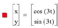
1.
Graph
y = sin ( t ) for 0 £ t
£ 2p
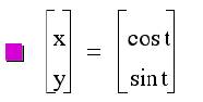
As you observe the
solution appears to be a circle with center at the orogin and a radius of 1.
Further, let us observe
the parametric equations
x = cos ( at )
y = sin ( bt ) for 0 £ t
£ 2p
for various a’s and b’s.
Let us observe some
examples:
1) a = b
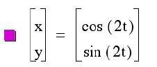
The observation is that although the values of a and b are changed
the circle remains about the origin with a radius of 1.
2)
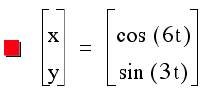
Let us observe what happens when we let a = 2 and we vary b in
each graph such that b = 3, then b= 4, then b=5, and finally b= 6.
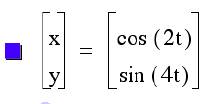
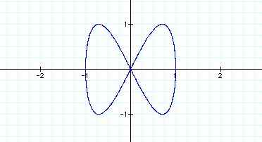
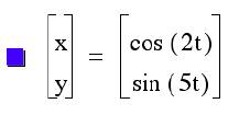
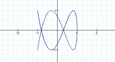
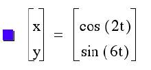
As we observe when a=2 ten the solution is a series of curves that
look like loops.
The number of loops depends on what the value of b is set at. The
number of loops = 1/2(b).
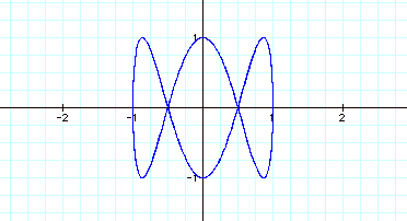
3)
This asks the question: what happens then when b= 2 and we vary a as we have
already done for b?
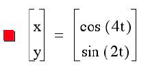

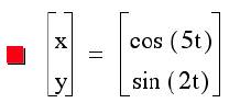

These graphs look very different; it appears that some of
the oddity is when a is an odd number versa a is an even number.
When a is an odd number, there is always 2 local maximums
and minimums for y and there is maximum and minimum for x.
When a is an even number, there
appears to be only one maximum and minimum for y and 1/2 of a maximums and
minimum for x.
When a=4, however, this is not true.
Could there be a relationship change since at that point a=2b.
4)
Let us observe what happens then when a=2b.


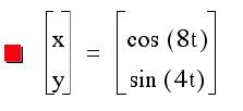
It seems true that when
a=2b the graph is always in the above shape.
Conclusion:
This investigation
shows a small sampling of what can be determined with the use of parametric
curves. There are many interesting investigations that we could continue with
yet this surely provides enough such that every new observation opens the doors
to many other variations.
Simple using the basic
curves and varying the a and b parameters to observe how the curves react provides us
with much more that can be used and expanded on in the classroom.