Robin Kirkham, Cara Haskins , and Matt Tumlin

____________________________________________________________

Let us examine the parabola as the coefficient values change to see the effects these changes have on the various parabolas.

Given the parabola y = ax² +bx +c with variables of a, b, and c.

Our first step is to :

Look at the basic parabola when a=1, b=0, and c=0

Notice that the domain is the set of all real numbers and the range is all non-negative numbers. The range for this basic parabola is all non-negative numbers.

The lowest point on a parabola is called the Minimum. The minimum point for our basic parabola is (0,0).

___________________________________________________________________

Continue to use the basic quadratic function as our frame of reference. Let us examine what happens to the graph under the following guidelines.

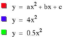
Step 1: y = ax²

Let b=0, c=0, and vary the values of a. Our new equation becomes y = ax².

Let us use the graphing calculator to examine the effects of varying the values for ‘a’, remembering to use both positive and negative values.

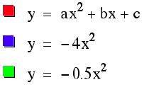
The red graph is y = ax2 +bx +c. y = ax², the basic parabola will always be in red in future examples for comparison purposes.

Notice that when the value for variable ‘a’ is positive, the minimum of the graph does not change even though the value for variable ‘a’ was changed. When a> 1, the graph has been narrowed horizontally, resulting in a horizontal shrinking of the graph. When 0< a< 1, the graph has now been stretched horizontally. This leaves the question as to what happens when negative values are substituted for variable ‘a’.

By substituting negative values for variable ‘a’, notice there is a reflection across the x-axis for our parabolas. The highest point on a graph is called a maximum. The maximum for our parabolas is (0,0).

Step 2: Now we are examining the effects of variable ‘b’. Let a=1, and c=0 and change the values for variable ‘b’. Our new equation is now y = ax² +bx .

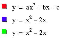
Notice that the widths of the parabolas remained the same while the location of the minimum changed. This movement appears to be equal to the value of ‘-c/2’, both vertically and horizontally. This is investigated in our step 3 below.

Step 3: Let us again start with equation y = ax² +bx +c. Let a=1, b=0, and vary c, resulting in y = ax²+c. Note that this investigation is not complete until we review the effects that variable ‘b’ my have with respect to variable ‘c’.

The value of variable ’c’ moves the parabola shifts up and down with respect to the y-axis. When c > 0, the graph moves up. When c < 0, the graph moves down.

This vertical movement changes with respect to our minimum point. This vertical shift appears to be equal to the value of variable ‘c’.

This shows that the horizontal and vertical shifts are a result of both the variables ‘b’ and ‘c’. The horizontal shift still appears to be negative ‘c/2’ while the vertical shift appears to be smaller than ‘c’. To be sure let us investigate further all three variables with respect to each other.

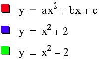
This investigation provides a very complicated graph, so it has been presented both separated as follows immediately and later all six parabolas together.

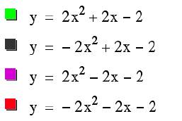
This first set of four parabolas demonstrates the results of modifications that are made to both the variables 'b and c' simultaneously.

The direction the parabola opens is related to the variable 'c' being positive or negative (positive - opens up and negative -opens down).

This shows us that the horizontal and vertical shifts are a results of all a, b, and c respectively. The horizontal shift turns out to be ‘-b/2a’.

When both values for variables ' b and c' are positive the parabolas are in quadrants I and II (positive on the y-axis).

It is interesting to view these two parabolas with their line of symmetry.

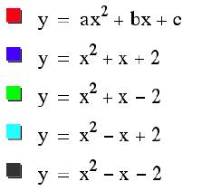
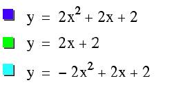
The following graph shows all six parabolas together. As we have observed these parabolas are perhaps better examined separated but it is useful for all of them to be viewed together.

This set of parabolas introduces many interesting effects.

Firstly, one can see that the y = ax² +bx +c where a, b, and c are all positive and the similar parabola where ‘a’ is the additive inverse, one observes that these two parabolas are inverses and both shifted to opposite quadrants around the line of symmetry y=2x+2 .

___________________________________________________________________

In summary, given the equation y = ax2 +bx +c the following are true:

Changes with the value of variable ‘a’ the direction the parabola opens (either up or down).

Changes with the value of variable ‘b’ effects the placement of the parabola in a horizontal shift (along the x-axis).

Changes with the value of variable ‘c’ effects the placement of the parabola in a vertical shift (y-axis).

Changes in the value of variable ‘c’ in conjunction with the value of variable ‘b’ together effects that phase shift of the graph. The three variables provide a complicated interaction with each other.

Return to Robin’s Homepage