
By
Ken Montgomery
An investigation of
Equation 1: ![]()
Letting a = 4, we have Equation 2.
Equation 2: ![]()
Plotting this relation (Figure 1)
yields a curve that does not pass the vertical line test and is therefore not a
function. We notice that the yintercepts are at 1, and 1 and that the
xintercepts are at 2 and 2 and that the graph passes through the origin.
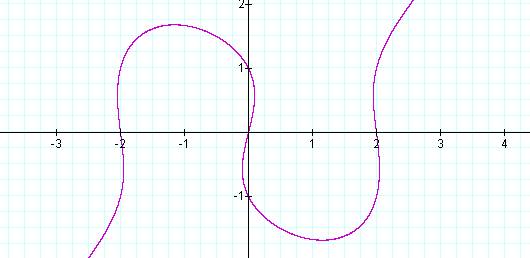
Figure 1: Graph of ![]() ,
with a = 4
,
with a = 4
By
increasing the value of a, from a = 4 to a = 5, we obtain
Equation 3.
Equation 3: ![]()
Again, plotting this relation we
obtain a curve of the same general shape, passing through the origin and
through the yintercepts 1 and 1. However, we notice that the absolute value
of the xintercepts has increased (i.e. the xintercepts have moved away from
the origin, Figure 2). From the graph in Figure 2, we approximate the
x-intercepts to be -2.25 and 2.25 as points of reference for comparison.
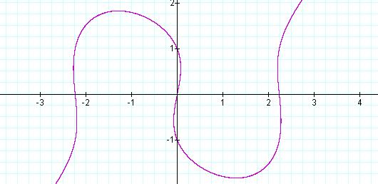
Figure 2: Graph of ![]() ,
with a = 5
,
with a = 5
Again
we change the value of a, from a = 5 to a = 3, yielding
Equation 4.
Equation 4: ![]()
Again, also we observe that the
curve continues to pass through the origin and through the y-intercepts, 1 and
1 (Figure 3). However, the absolute value of the x-intercepts has decreased
from 2.25 to 1.75.
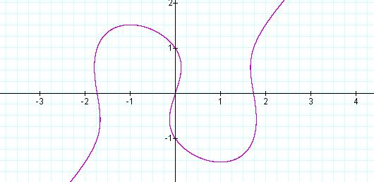
Figure 3: Graph of ![]() ,
with a = 3
,
with a = 3
With a = 2, we have Equation 5 and
we see from the graph (Figure 4) that the x intercepts are approximately 1.4
and 1.4 respectively. The bends in the curve (located in the areas of (-1.25,
-3) and (1.24, 3)) have become more pronounced and seem to be approaching x =
0, as a approaches zero.
Equation 5: ![]()
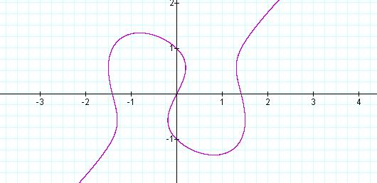
Figure 4: Graph of ![]() ,
with a = 2
,
with a = 2
Finally, we let a = 1, obtaining
the graph of Equation 6, in Figure 5.
Equation 6: ![]()
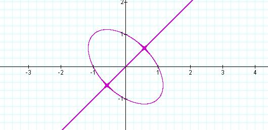
Figure 5: Graph of ![]() ,
with a = 1
,
with a = 1
The figure seems to be a graph of
an ellipse and the minor axis, y = x. The composite graph of these combined
functions is given in Figure 6, by Equation 7.
Equation 7: ![]()
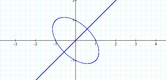
Figure 6: Graph of ![]()
We can show that these graphs are
in fact identical by factoring Equation 6 into Equation 7.
![]()
![]()
![]()
![]()
![]()
![]()
Ò
We wish to examine the graph for values of a close to 1, so we first let a = 1.1, obtaining Equation 8. We then let a = 0.9, to obtain Equation 8, and compare the graphs in Figure 7 and in Figure 8.
Equation 8: ![]()
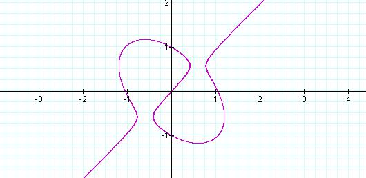
Figure 7: Graph of ![]() ,
with a = 1.1
,
with a = 1.1
We see that as a decreases,
the vertical openings in the graph at a = 1.1 close at a = 1 and
then open horizontally at a = 0.9.
Equation 9: ![]()
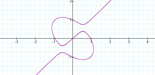
Figure 8: Graph of ![]() ,
with a = 0.9
,
with a = 0.9
We then explore the effect on the
graph of negative a values. Letting a = -3, we have Equation 10,
and the graph in Figure 9. We still have a graph passing through the origin and
with y-intercepts at y = -1 and y = 1. The curves are much less pronounced now,
with the openings horizontal.
Equation 10: ![]()
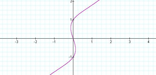
Figure 9: Graph of ![]() ,
with a = -3
,
with a = -3
For a = -1 (Equation 11, Figure 10)
the curve becomes more pronounced.
Equation 11: ![]()
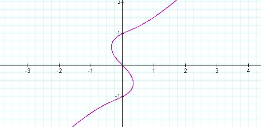
Figure 10: Graph of ![]() ,
with a = -1
,
with a = -1
As a
approaches zero from the left, with smaller and smaller negative values, we
observe behavior similar to that in Figures 1-3, but about the y axis, as
opposed to the x axis.
Equation 12: ![]()
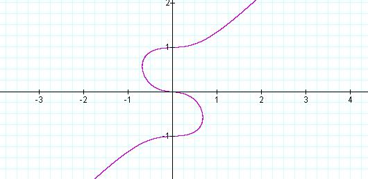
Figure 11: Graph of ![]() ,
with a = -0.1
,
with a = -0.1
An animation of the relation was created for a = n, with 10 < n < 10.
Heres a link to the movie Assign1KM.avi
It may then be apparent that for
each value of a, we are viewing a different cross-section, or contour
map of a relation which could be plotted in three dimensions, for Equation 13.
Equation 13: ![]()
Heres a link to the movie Assign1KM3D.avi
We next add a constant to the left
side of Equation 2, to obtain Equation 14.
Equation 14: ![]()
We animate the graph by varying n between its bounds: 10 < n < 10.
Heres a link to the Assign1xKM.gcf file for this equation
Investigating the same behavior for
the function with a constant added to the left side, we have Equation 15.
Equation 15: ![]()
Again the graph is animated, with 10 < n < 10.
When n = 2, we have Equation
16, the graph of which is given in Figure 12.
Equation 16: ![]()
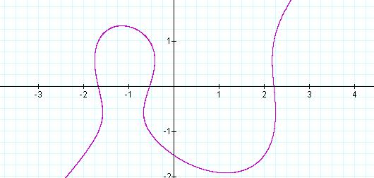
Figure 12: Graph of ![]() , with a = 4 and n = 2
, with a = 4 and n = 2
Heres a link to the Assign1yKM.gcf file for this equation
Return to Homepage