
In this study, Graphing Calculator 3.2 is used to investigate equations of conic sections in polar form. The eccentricity e is represented by k, since Graphing Calculator only recognizes e as the base of the natural logarithm function. Eccentricity is a number describing the shape of a conic section, and is equal to the quotient of the distance from the curve to the focal point and the distance from the curve to the directrix. For the ellipse described in the Cartesian coordinate system by the Equation 1.
Equation 1: ![]()
The eccentricity (k) is given by Equation 2.
Equation 2: ![]()
However, we are working with polar coordinates and the equation for our parabola, is given by Equation 3.
Equation 3: ![]()
For the case
when k = 1, we have the graph in Figure
1.
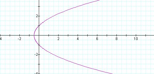
Figure 1: Graph of ![]() , k =1, p = 1
, k =1, p = 1
If the cos(h) is changed to a sin(h), we have Equation 4.
Equation 4: ![]()
This graph is also a parabola, but
rotated -![]() radians
about the origin. This rotation corresponds to the
radians
about the origin. This rotation corresponds to the ![]()
phase
difference between cosine and sine (Figure 2).
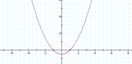
Figure 2: Graph of ![]() ,
k =1, p = 1
,
k =1, p = 1
If this equation is changed to Equation 5,
Equation 5: ![]()
we get the same graph as Figure 1,
but rotated ![]() radians
about the origin (Figure 3).
radians
about the origin (Figure 3).
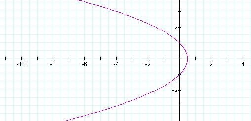
Figure 3: Graph of ![]() ,
k =1, p = 1
,
k =1, p = 1
Once again, however if the cos(h) is changed to a sin(h), the equation changes and we get Equation
6.
Equation 6: ![]()
The graph is identical to those
already presented, but rotated -![]() radians
about the origin, with respect to the
radians
about the origin, with respect to the
graph in Figure 3 (see Figure 4).
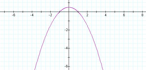
Figure 4: Graph of ![]() ,
k =1, p = 1
,
k =1, p = 1
Either adding or subtracting the sine or cosine function therefore will change the orientation of the conic section in question. For the current values of p = 1 and k = 1, however we see that the graph is a parabola. The eccentricity, k, however may be changed, for the first equation (Figure 1) with p held constant.
We investigate for
the case, k < 0 and we have the
identical graph of the parabola in Figure 1, for the case when k = -1 (Figure 5).
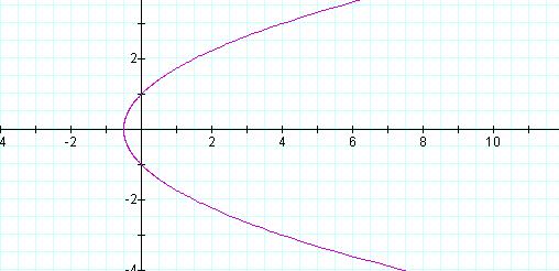
Figure 5: Graph of ![]() , k = -1, p = 1
, k = -1, p = 1
However, if k is chosen such that 1 < k < 0, we have an ellipse. An example, with k = 0.9 is given in Figure 6.
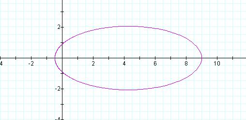
Figure 6: Graph of ![]() , k = -0.9, p = 1
, k = -0.9, p = 1
If the eccentricity is increased to
k = -0.5, a smaller ellipse is graphed
(Figure 7).
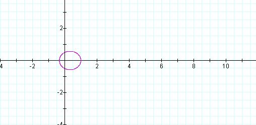
Figure 7: Graph of ![]() , k = -0.5, p = 1
, k = -0.5, p = 1
This is
interesting, as the eccentricity has not gotten smaller as 0.9 < -0.5.
However, the absolute value of the eccentricity, k, has been reduced. Further, the exact same graph is
also obtained for k = 0.5. To
investigate the case for k >
1, we set k = 1.5 and obtain the
graph in Figure 8.
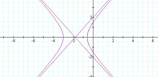
Figure 8: Graph of ![]() , k = 1.5, p = 1
, k = 1.5, p = 1
Although we might have been tempted to assume that an ellipse will be produced for non-integer, rational numbers, we see that k must be bounded as 0 < |k| < 1. We instead obtain a hyperbola, with the asymptotes provided by Graphing Calculator©. To better understand the transitions between, and beyond these values of k, we set the value equal to n and animate the graph for 10 < n < 10 to obtain Movie11KM. As n varies, we see the transition from hyperbola, to ellipse, to parabola, and back to hyperbola. We see that eccentricity, therefore determines the conic section described by the general form of the equation. We now turn our attention to the effect of changing p.
If for the same
equation, we vary p, with k held constant, we notice that the size of the conic
section appears to change, but not the conic section itself. For the case of
the ellipse, we let k = -0.5 and
change the value from p = 1 to p = 2 (Figure 10). The distance from the directrix to
the focus is represented by p,
thus a change in p results in a
change in this distance.
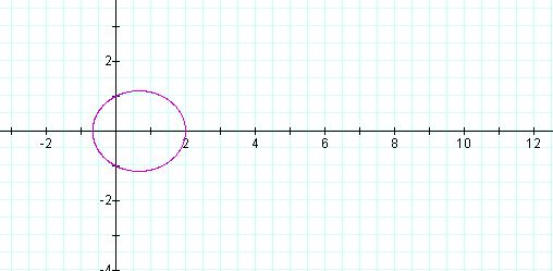
Figure 10 Graph of ![]() , k = 0.5, p = 2
, k = 0.5, p = 2
A comparison of Figure 7 and Figure 10 will verify that the ellipse given by p = 2 appears to be twice as large. This same exploration will verify for cases, these same results for parabola and hyperbola.
Setting
k = 1, we do not get the parabola of
Figure 1 with p =2 (Figure 11).
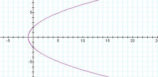
Figure 11 Graph of ![]() , k = 1, p = 2
, k = 1, p = 2
Instead we get a parabola that intersects the y-axis at y = 2 and y = -2 as opposed to y = 1 and y = -1. The parabola still, however passes through x = -1.
We have a similar parabola (eccentricity, k is held constant), but twice the size (p is doubled).
To observe this effect for the
hyperbola, we change the p value from p = 1 to p
= 2 for the equation given in Figure 8 (see Figure 12).
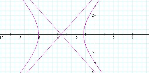
Figure 12 Graph of ![]() , k = 1.5, p = 2
, k = 1.5, p = 2
A comparison of Figure 8 and Figure 12 verifies that the distance from the directrix to the focus has doubled.
In closing, we see that a conic
section whose focus is at the origin, with directrix ![]() , and with eccentricity k has polar the form given in
Equation 7.
, and with eccentricity k has polar the form given in
Equation 7.
Equation 7: ![]()
If the directrix is ![]() , its graph is given by Equation 8.
, its graph is given by Equation 8.
Equation 8: ![]()
For k<1, the graph is an ellipse; for k=1, it is a parabola; and if k>1, it is a hyperbola.
Return to Homepage