
EMAT6680 Assignment 3
Quadratic and Tertiary Equations
By Kevin Perry
More on Quadratic
Equations and Parabolas
In our last discussion, we discovered that for a quadratic equation represented as a function of y,
![]()
that if you fix A and C and vary B, you get the graph
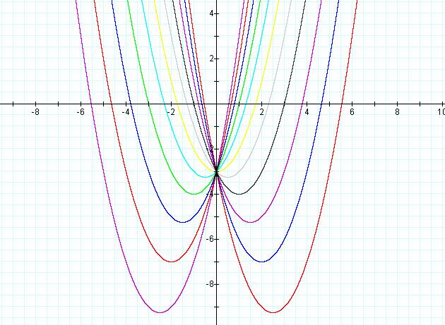
In the graph, we notice that the locus of the vertices of the parabolas makes a shape that is quite similar to a parabola (facing down). We would now like to prove that this locus is in fact a parabola, and discover a general form of that parabola.
The curves in the graph above are all of the form
![]()
We can note from the graphs (or from calculus) that the vertex of any one curve is located at the point where

and
if we then note that y can be written as
we can substitute x in for –B/2 and get
![]()
If we then add this function to the above graph, we get
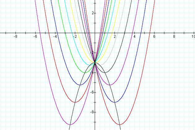
To generalize this formula for the locus of the vertices of the changing B term, we start with the general formula
![]()
take the derivative with respect to x and set it equal to zero to find the maximum(minimum) point
![]()
and solve for x to get
to get the y value at that point, we substitute back into the original equation to get
which solves to
and then we can substitute x back in for –B/2A and get
![]()
as the general formula for the locus of vertices of the parabola as B changes.
Exploration of the
changing quadratic terms
Now that we have seen that the vertex of the parabola can be defined as the B term of a quadratic equation changes, we could investigate further into how these changing terms can affect the roots of the quadratic formula
![]()
For example, if we are changing B, how does that affect solving for the roots of the equation?
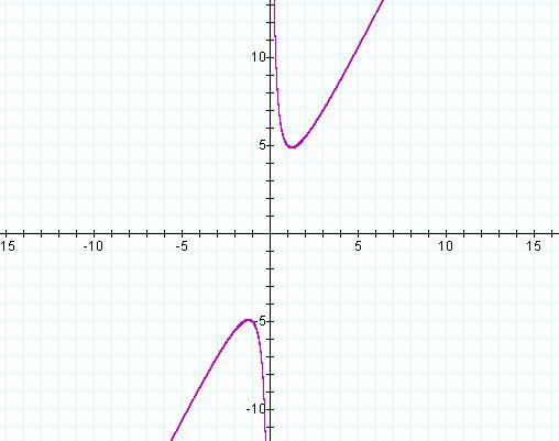
To study this, we must first think of the equation as B(x), in other words, B as a function of x. For our discussion, let’s set A=-2 and C=-3, so that the equation is now
![]()
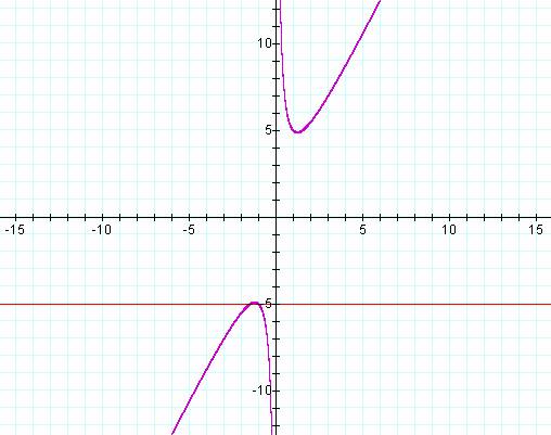
The graph of this equation is
We can also add another graph to the equation that represents a particular value of B, for example B=7
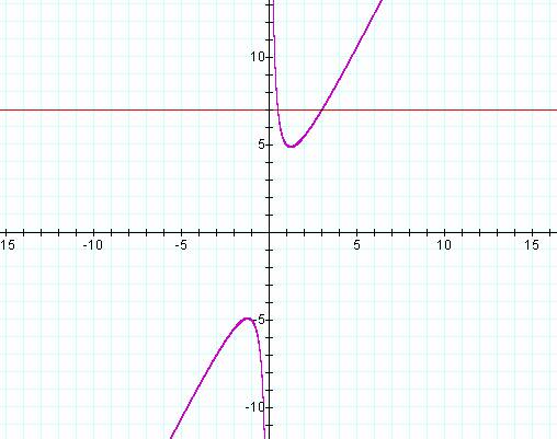
We see from that line that B=7 intersects
![]()
at two points, and both of those points are on the positive side of the x axis. This means that the roots of the equation are both positive and are real roots. The intersection points are in fact the roots of the equation
![]()
From the graph, they are x=3 and x=1/2. Next, let’s look at B=3.
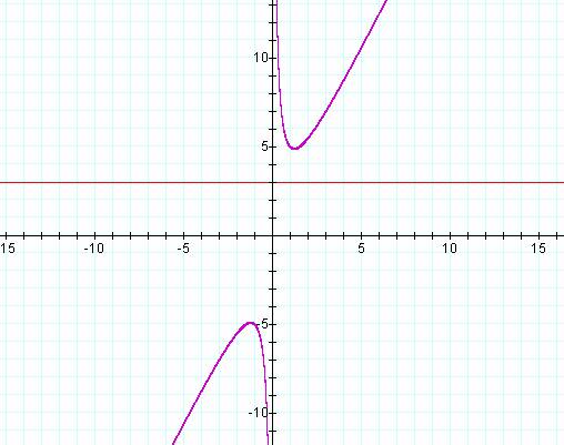
The line and the curves do not intersect at all. Therefore there are no real roots to the equation
![]()
Next, let’s look at B=-5
We can see from the graph, that somewhere close to B=-5, the line will intersect the curves at exactly one point. At that value of B, there are two real roots of the equation, but both roots have the same value (or the solution is a double root). The exact value for B that gives a double root is the square root of 24 (approximately 4.8989795) and the double root is at approximately 1.2247449.
So to summarize what we can gather from the graph, the equation
![]()
will have two negative real roots for B<4.899, it will have a double root at approximately B=-4.899 and B=4.899, it will have no real roots for -4.899<B<4.899, and it will have two positive roots for B>4.899.
These graphs can be generalized for different values of A and C. An example for different values of C is
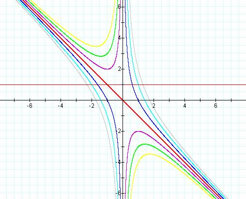
For each of the values of C, we can define the range of values for B that will give real roots.
Explore some quadratic equations.
Extension to
tertiary equations
The next logical extension to this analysis of roots of equations is third order equations of the form
![]()
If we set the constants, we could have
![]()
Graphing the left hand side of the equation as a function, we get
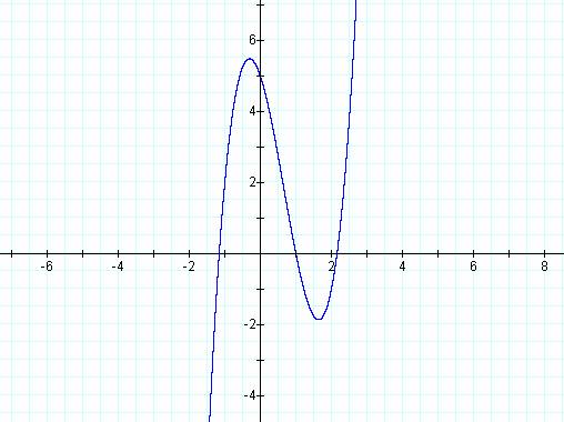
We can see that there are three roots to the equations based on the three points that intersect the x axis.
But now we want to investigate how changing the different coefficients of the equation change the roots of the equation.
If we want to change the B term, we can compute the graphs in the XB plane. First, take our equation and set the B term back to B
![]()
If we make some graphs of the equation with different B, we get
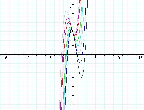
We can see that for different B, the roots are different, but how can we explain how they change for the different B? We can change the graph to the XB plane, and see the following graph
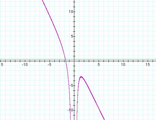
If the green line represents the value of B for a particular equation, the intersection of the line and the curve in the XB plane represents the roots of the equation. From our earlier discussion, we can see that as B varies, the roots go from one real (negative) root, to one negative real root and a positive double root, and finally to one negative real root, and two positive real roots. If you correlate the two previous graphs, you can see the relation between the value of B and where the curve for the equation crosses the x axis.
Conclusions
What we have learned in this discussion is that by manipulating the graphing of equations in different parameter planes, we can discover more properties of the roots of quadratic and tertiary equations. This method can be used for any type of equation that can be simplified into coefficient terms. The exploration of these different graphs can very clearly demonstrate the properties and interconnections of the roots of equations.