Boiling Water

Janet Shiver

EMAT 6680

Investigation: Take a cup of boiling water and measure its initial temperature. Then record the temperature of the water each minute for thirty minutes. Graph the data and then construct a function to model the data. Calculate a measure of the error between the model and the observed data. Finally, using the function, predict the temperature after 45 minutes, 60 minutes, or 300 minutes.

Collect the Data

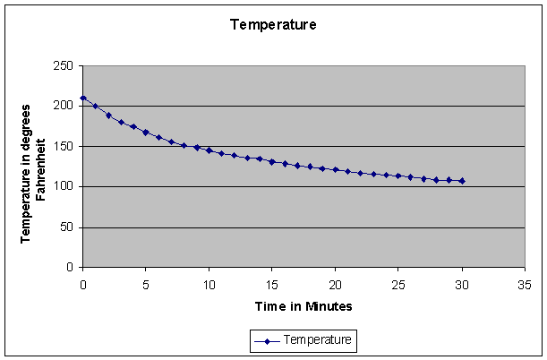
After boiling a cup of water, I recorded its temperature every minute for thirty minutes. The data is graphed below, with the independent variable as time in minutes and the dependent variable as temperature.

Time	Temperature

0	210
1	200
2	189
3	180
4	174
5	167
6	161
7	156
8	151
9	148
10	145
11	142
12	139
13	136
14	134
15	131
16	128
17	126
18	125
19	123
20	121
21	119
22	117
23	116
24	114
25	113
26	112
27	110
28	109
29	108
30	107

Finding a model

Our next task will be to develop a model for this data. We must attempt to find a cooling function that will “best” fit our data. As we do this, we must keep in mind that since our data is “real-world” it is highly unlikely that we will be able to find a curve that matches it exactly. We need to focus instead on finding a function that will best match our data.

We will begin by first examining the general shape of the graph and its behavior. Several basic functions can be eliminated based on the appearance of the graph. The graph of the data does not lie on line so the linear function can be eliminated as a possibility. It is also does not resemble a parabola so the quadratic function would not be a good choice. We can also eliminate the cubic function and higher order polynomials for the same reasons of appearance. So we can safely say that the graph does not resemble any polynomial functions. It is also safe to eliminate the trigonometric functions since the graph has no periodicity.

The function that the graph most closely resembles is the exponentional decay function. As with all exponential decay models, our graph shows a rapid decrease at the beginning of the time. As time progresses, the graph continues to decrease in temperature but at a much slower rate. We could conjecture that if we continued to take readings that the water would ultimately reach room temperature which in this case was 77 degrees.

Exponential Decay Model

The general form of any exponential model is , where a is the initial value at time 0, k is the decay constant, and t is time in minutes. We will use an excel spread sheet to try to find an appropriate model. The model that I first tried was . I let a = 210 since this was the boiling point of my water. I found k using an excel spreadsheet and good old trial and error. You can see the y values that my model produced in the chart below along with the squares of the differences between the actual data and the values produced by my model.

Time	Temperature	*y=210e^(-.028t)**	Square of the difference

0	210	210.00	0.00
1	200	204.20	17.65
2	189	198.56	91.46
3	180	193.08	171.10
4	174	187.75	189.04
5	167	182.57	242.28
6	161	177.52	273.05
7	156	172.62	276.31
8	151	167.86	284.13
9	148	163.22	231.69
10	145	158.71	188.09
11	142	154.33	152.08
12	139	150.07	122.56
13	136	145.93	98.55
14	134	141.90	62.38
15	131	137.98	48.72
16	128	134.17	38.07
17	126	130.47	19.94
18	125	126.86	3.47
19	123	123.36	0.13
20	121	119.95	1.09
21	119	116.64	5.56
22	117	113.42	12.81
23	116	110.29	32.61
24	114	107.24	45.64
25	113	104.28	75.99
26	112	101.40	112.29
27	110	98.60	129.88
28	109	95.88	172.11
29	108	93.23	218.05
30	107	90.66	267.02

Sum of the squares	3583.74918
	119.458306

By calculating the difference between my model and the actual data using the least squares method we can see that our model needs to be improved on. 119.46 is much higher than we would like; we would prefer that the difference between the actual data and the model be much closer to zero.

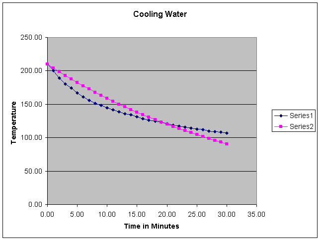
Now lets look at it graphically.

We can see that our model does not fit the curve of the actual data well. Although our model is decreasing it is decreasing too slowly for the first 20 minutes and then too quickly during the last 10.

How can we improve this model? We must now consider that most decay models approach the value of zero but this is not the case for our model. This experiment was conducted in a room that was 77 degrees so once our water cools completely it should maintain a temperature of the air in the room or 77 degrees.

We must now consider Newton’s Law of Cooling. Newton’s law of cooling states that the final temperature of an object that is warmer than the air around it will be the room temperature. This temperature can be determined by the formula , where is the final temperature, is the initial temperature and is the room temperature.

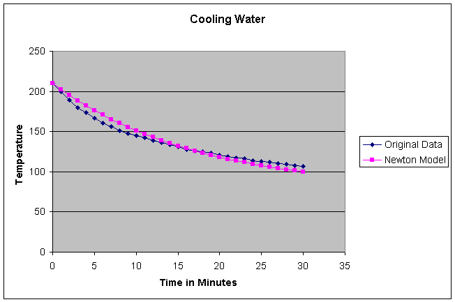
The model we will use is . You can see from the sum of the squares of the difference that, at 34.72, we were much closer to zero this time. You can also see from the graph that our model appears to have the same general shape as our original data.

Time	Temperature	y =77+133e^(-.0586t)	Square of the Difference

0	210	210.00	0.00
1	200	202.43	5.91
2	189	195.29	39.58
3	180	188.56	73.25
4	174	182.21	67.39
5	167	176.22	85.03
6	161	170.57	91.66
7	156	165.25	85.52
8	151	160.23	85.10
9	148	155.49	56.07
10	145	151.02	36.25
11	142	146.81	23.12
12	139	142.83	14.71
13	136	139.09	9.53
14	134	135.55	2.41
15	131	132.22	1.49
16	128	129.08	1.16
17	126	126.11	0.01
18	125	123.32	2.83
19	123	120.68	5.37
20	121	118.20	7.86
21	119	115.85	9.91
22	117	113.64	11.29
23	116	111.55	19.76
24	114	109.59	19.46
25	113	107.73	27.74
26	112	105.98	36.19
27	110	104.33	32.10
28	109	102.78	38.70
29	108	101.31	44.74
30	107	99.93	50.02

Sum of the squares 1041.616

34.72

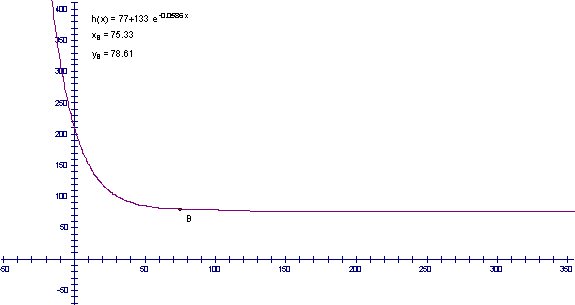
Lets use our model to predict the temperature at 45, 60 and 300 minutes. Click here to see the model. Move point b to determine the temperature at any given time. Pay attention to the temperature as the time increases and record your results for 45 minutes, 60 minutes and 300 minutes.

Scroll Down For The Solutions

Solutions: 45 minutes - 86 degrees, 60 minutes - 81 degrees, and 300 minutes - 77 degree

Did you notice that as the time increased the temperature went to room temperature, 77 degrees. For further investigation you might want to determine when the model first reached 77 degrees and what this means. You might also want to investigate whether the model will drop below 77 degrees and when this occurs.

Return to Janet Shiver’s Home Page