Parametric Equations

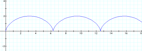
We can often use graphs to explore parametric equations. Let's begin with the graphs of

We can see that the graph is a circle. What if we multiplied our equations by a constant?

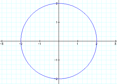
We can see that is simply increases the radius of our circle. Now what if we added a constant to our equation?

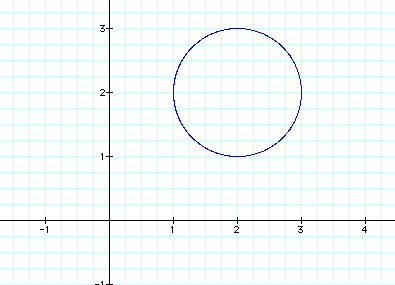
We can see that it simply moves the center of our circle. What if we multiplied t by a constant. Lets consider the equation

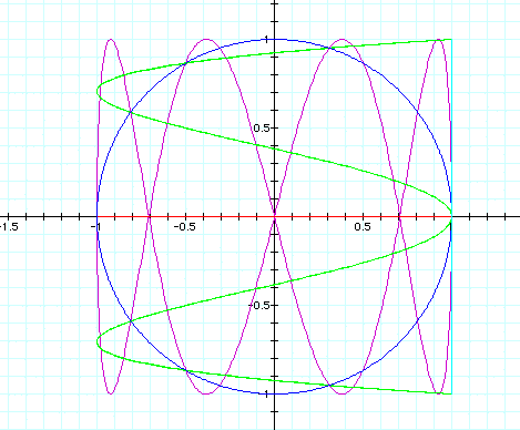
The blue graph is our original equation. The red graph has a=1 and b=0, and the light blue graph has a=0 and b=1. The green graph has a=4 and b=1, and the purple graph has a=1 and b=4.

Click HERE to see the animation of a as we hold b constant. Or click HERE to see the animation of b as we hold a constant.

What if we changed our equation to read

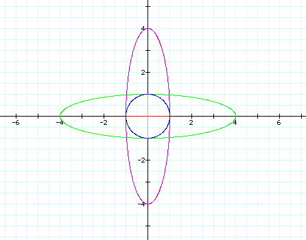
Again the blue graph is our original equation. The red graph has a=1 and b=0, and the light blue graph has a=0 and b=1. The green graph has a=4 and b=1, and the purple graph has a=1 and b=4.

Click HERE to see the animation of a as we hold b constant. Or click HERE to see the animation of b as we hold a constant.

We can also explore the equations and .

When we graph them they look very similar to our original set of equations .

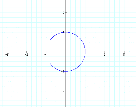
What if we added constant terms, a and b, in front of each t.

and

Again the blue graph is our original equation. The red graph has a=1 and b=0, and the light blue graph has a=0 and b=1. The green graph has a=4 and b=1, and the purple graph has a=1 and b=4.

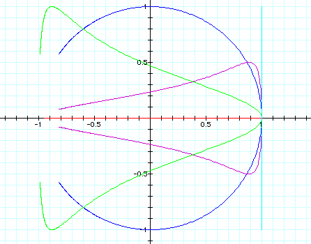
Now lets graph several graphs for the following equations.

We will begin with k=1. Now the blue graph is a=1 and b=1. The purple graph has a=1 and b=0 , and the red graph has a=0 and b=1 . The green graph has a=4 and b=1 , and the light blue graph has a=1 and b=4 . The yellow graph has a=0 and b=0.

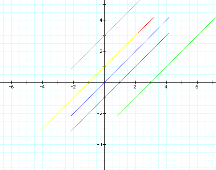
We can see they are all paralell straight lines. Click HERE to see the animation of a as we hold b constant. Or click HERE to see the animation of b as we hold a constant. Now what happens as we change k. Lets hold a and b constant, and click HERE to see the graph as k changes.

Now lets see the graph of .

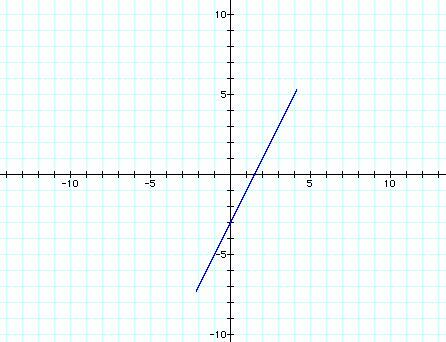
If we want to write parametric equations of a line segment through (7, 5) with slope of 3, we can interpret the previous graphs to see that the slope is the coefficient of t in the y equation divided by the coefficient of t in the x equation, and the y intercept is the negative slope times any summand in the x equation plus any summand in the y equation. So for an equation with slope of 3, we know y=3t plus something. If we want the segment to go through (7,5) we can use 7 and 5 for our respective summands in the equations. So we have

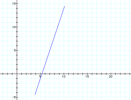
Now lets return to the equation

If we look at our graphs again were the blue graph is our original equation, the red graph has a=1 and b=0, the light blue graph has a=0 and b=1, the green graph has a=4 and b=1, and the purple graph has a=1 and b=4, we can conclude that the graph is a vertical ellipse when a<b and a horizontal ellipse when a>b and a straight line when either a or b are zero (vertical when a=0 and horizontal when b=0), and a circle when a=b. Now lets change the equation again to the following

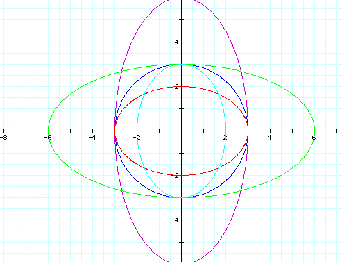
Now lets hold a and b constant at a=b=1 and click HERE to see the graph as h changes. What if a>b, or a<b? Click HERE to see the graph as h changes when a=4 and b=1, or click HERE to see the graph as h changes when a=1 and b=4.

We can see that the graph is usually just stretched horizontally or vertically when a>b or a<b. Lets explore some other equations and see if this assumption holds true. First we will look again at

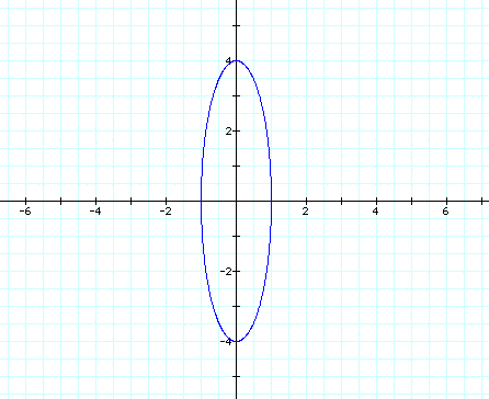
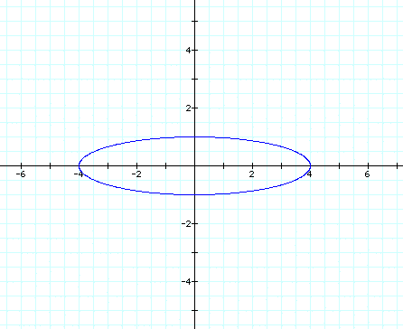
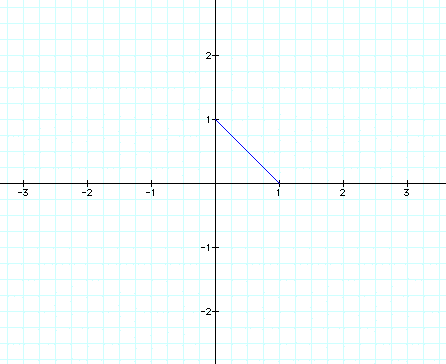
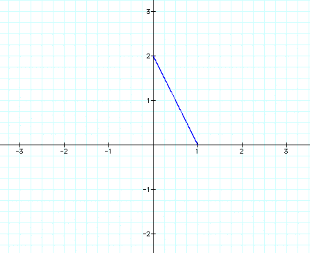
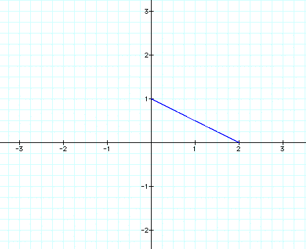
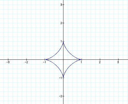
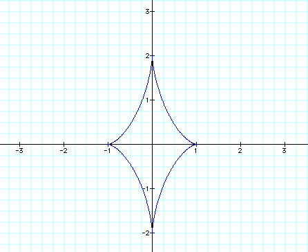
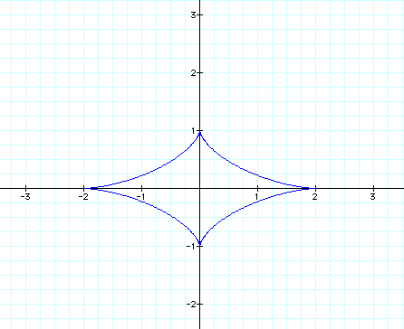
So our assumption was correct, when a<b the graph is stretched vertically and when a>b the graph is stretched horizontally.

Now lets consider the equation . If we want to put this equation into parametric equations we could let y=tx cross the curve at (0,0) and at (x,y). Then, substituting, and then we have the parametric equations

When we graph the two equations, we can see they are almost identical.

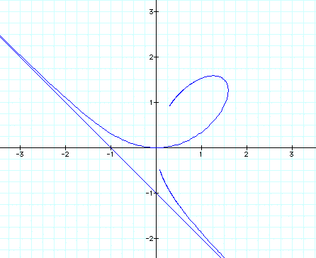
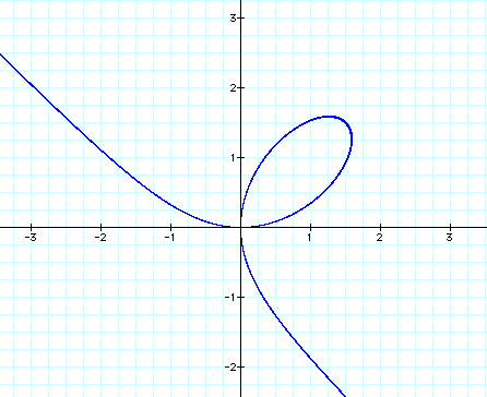
Now lets look at the equations below with the following values for a and b.

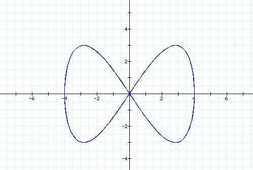
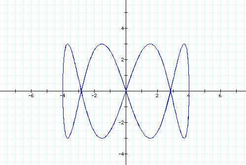
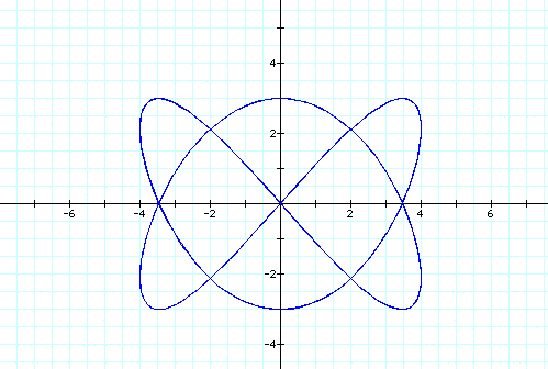
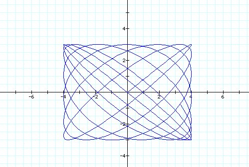
We notice that no matter what values we plug in for a and b our graph is always restricted between 4 and -4 on the x-axis and between 3 and -3 on the y-axis. This class of parametric curves are called the Lissojous curves. Now lets compare them to the graphs of

for the same values of a and b.

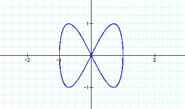
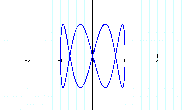
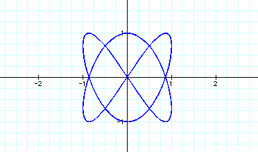
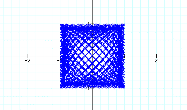
The graphs are the same as the Lissojous curves except they are restricted between -1 and 1 both vertically and horizontally.

Now if we define a cycloid as the locus of a point on a circle that rolls along a line, we can write a parametric equation for a cycloid of a circle with radius 1. Click HERE to see a GSP animation of the creation of the cycloid.