We will first begin by looking
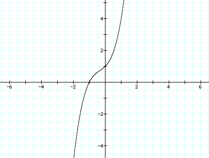
at the equation ![]() . We can look at
the graph below of
. We can look at
the graph below of ![]() . And we can also
hold one variable constant and see how the graph
varies as we change the others.
. And we can also
hold one variable constant and see how the graph
varies as we change the others.
We can use the graphs to determine
the roots of the equation ![]() , as
three of the variables are held constant. For example in the graph
below we will hold a, c, and d constant at a=c=d=1 and graph several
values of b. The purple graph shows b=(-3), the red graph shows
b=(-2), the blue graph shows b=(-1), the green graph shows b=0,
the light blue graph shows b=1, the yellow graph shows b=2, and
the grey graph shows b=3.
, as
three of the variables are held constant. For example in the graph
below we will hold a, c, and d constant at a=c=d=1 and graph several
values of b. The purple graph shows b=(-3), the red graph shows
b=(-2), the blue graph shows b=(-1), the green graph shows b=0,
the light blue graph shows b=1, the yellow graph shows b=2, and
the grey graph shows b=3.
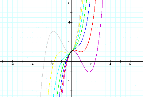
We notice that the graph always passes the y- axis at the point (0,1), and as the value of b increases the graph gets more extreme.
Now we can explore the equation
in the xb plane. By graphing our original equation, ![]() in the xb plane, we get the following graph.
in the xb plane, we get the following graph.
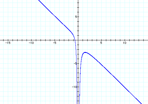
If we take any particular value of b, say b = 3, and overlay this equation on the graph we add a line parallel to the x-axis. If it intersects the curve in the xb plane the intersection points correspond to the roots of the original equation for that value of b. We have the following graph
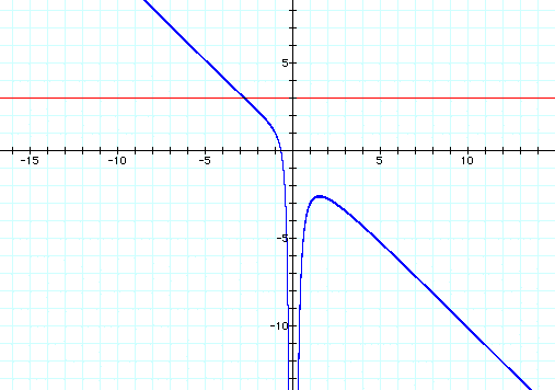
For each value of b we select, we get a horizontal line. It is clear on a single graph that we get two real roots of the original equation when b < -2, and two real roots when b > -2.
What would happen if we let c=-1 instead of c=1. We would get the following graph
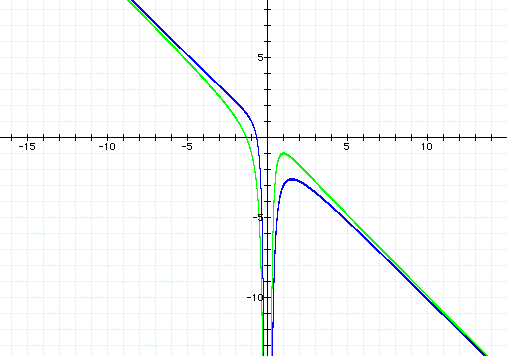
If we keep a and b constant the graph changes a great deal as we change c. We can see in the graph below a few different values of c. The purple graph shows c=(-3), the red graph shows c=(-2), the blue graph shows c=(-1), the green graph shows c=0, the light blue graph shows b=1, the yellow graph shows c=2, and the grey graph shows c=3.
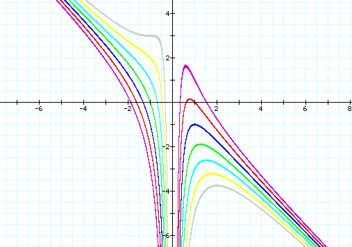
Or you can click HERE to see the animation of the graph as c changes.
Now we can explore the graph
in the xc plane. When we graph our original equation,![]() ,
in the xc plane, we get the following graph
,
in the xc plane, we get the following graph
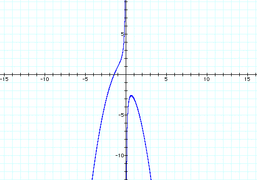
If we take any particular value of c, say c = -3, and overlay this equation on the graph we add a line parallel to the x-axis. If it intersects the curve in the xc plane the intersection points correspond to the roots of the original equation for that value of c. We have the following graph
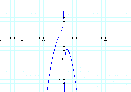
For each value of c we select, we get a horizontal line. It is clear on a single graph that we get three negative real roots of the original equation when c < -2.6, two positive real root when c = -2.6, and one real roots for c > -2.6.
What would happen if we let b=-1 instead of b=1. We would get the following graph
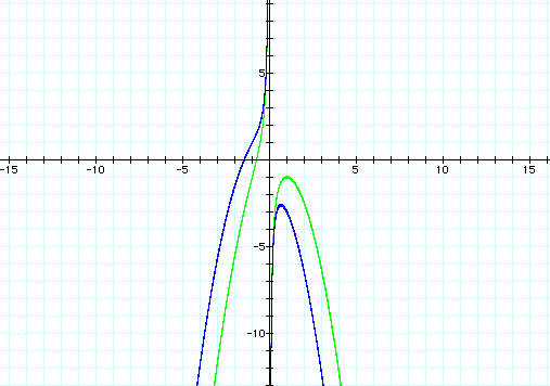
If we keep a, c and d constant the graph changes a great deal as we change b. We can see in the graph below a few different values of b. The purple graph shows b=(-3), the red graph shows b=(-2), the blue graph shows b=(-1), the green graph shows b=0, the light blue graph shows b=1, the yellow graph shows b=2, and the grey graph shows b=3.
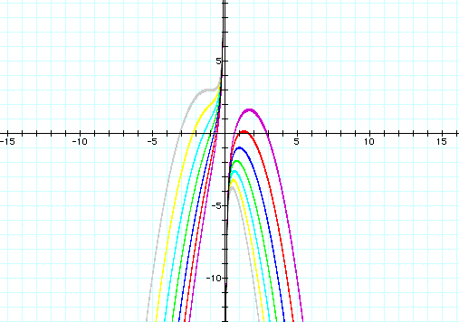
Or you can click HERE to see the animation of the graph as b changes.
Now we can explore the graph
in the xd plane. When we graph our original equation,![]() ,
in the xd plane, we get the following graph
,
in the xd plane, we get the following graph
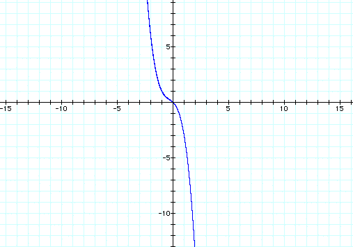
If we take any particular value of d, say d = -3, and overlay this equation on the graph we add a line parallel to the x-axis. If it intersects the curve in the xd plane the intersection points correspond to the roots of the original equation for that value of d. We have the following graph
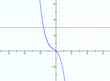
For each value of d we select, we get a horizontal line. It is clear on a single graph that we get one real roots of the original equation no matter what d is.
What would happen if we let b=-1 instead of b=1. We would get the following graph
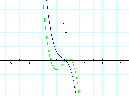
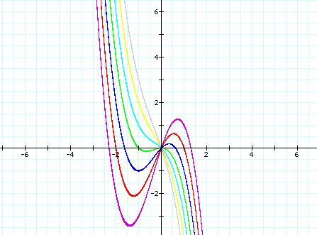
If we keep a, c and d constant the graph changes a great deal as we change b. We can see in the graph below a few different values of b. The purple graph shows b=(-3), the red graph shows b=(-2), the blue graph shows b=(-1), the green graph shows b=0, the light blue graph shows b=1, the yellow graph shows b=2, and the grey graph shows b=3.
Or you can click HERE to see the animation of the graph as b changes.