

For those who are not familiar with the history, linear programming is an optimization method developed during World War II for use in optimizing the allocation of labor and materiel critical to the war effort. Linear programming is now used on a wide scale in nearly all industries in a variety of fashions to optimally allocate labor, transportation, resources, etc. The purpose of this essay is to show how Geometer's Sketch Pad (GSP) can be used to enhance an introduction to linear programming in a classroom environment. The class of problems that can be demonstrated using GSP is limited because only two variables can be modeled. However, the basic concepts of linear programming can be easily understood from a two variable model. Actually, linear programming can be done graphically only in two or three variables, linear programming in more than three variables requires the use of special algorithms, one of which is the simplex algorithm, which can be found in any text on linear programming. (Linear programming in three variables requires that one be able to graph in three dimensions.) The basics of linear programming will be presented, then a small linear programming problem with two decision variables will be solve, both using GSP.
The decision variables in a linear programming model are those variables that represent production levels, transportation levels, etc. which are under the control of the decision maker(s).
With each decision variable there is associated a cost (loss) or a profit (gain) for each unit change in the variable. These values are represented by the Cost or Profit coefficients.
The objective function is an equation representing the profit (gain) or cost (loss) related to the decision variables. Objective functions take the one of the following forms:
![]()
The objective, of course is to maximize a profit objective and to minimize a cost objective.
If resources were unlimited, there would be no need to use LP. Because resources are limited the constraints on these must be modelled in some manner. This is done in the form of inequalities that describe mathematically the limitations on the resources. (Actually, constraints are not limited to inequalities, but, for demonstration purposes only inequalities will be used.) Normally, for a cost objective function the inequalities will be greater than or equal to, and for a profit objective the inequalities will be less than or equal to inequalities.
In LP models it is assumed that no variables may take on negative values, therefore each variable will have an associated constraint that limits it to values greater than or equal to zero.
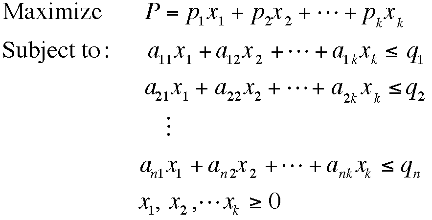
There are two basic LP models: the maximization model in standard form and the minimization model in standard form. An example of the former is shown below.
The following problem was taken from Finite Mathematics for Business, Economics, Life Sciences, and Social Sciences, Raymond Barnett, Michael Ziegle, and Karl Byleen, Prentice Hall, 1999.
Manufacturing --Resource Allocation. A furniture manyufacturing company manufactures dining room tables and chairs. The relevant manufacturing data are given in the table.
| Department |
Labor-Hours per Unit Tables |
Chairs |
Maximum Labor-Hours Available per Week |
| Assembly | 8 | 2 | 400 |
| Finishing | 2 | 1 | 120 |
| Profit per Unit | $90 | $25 |
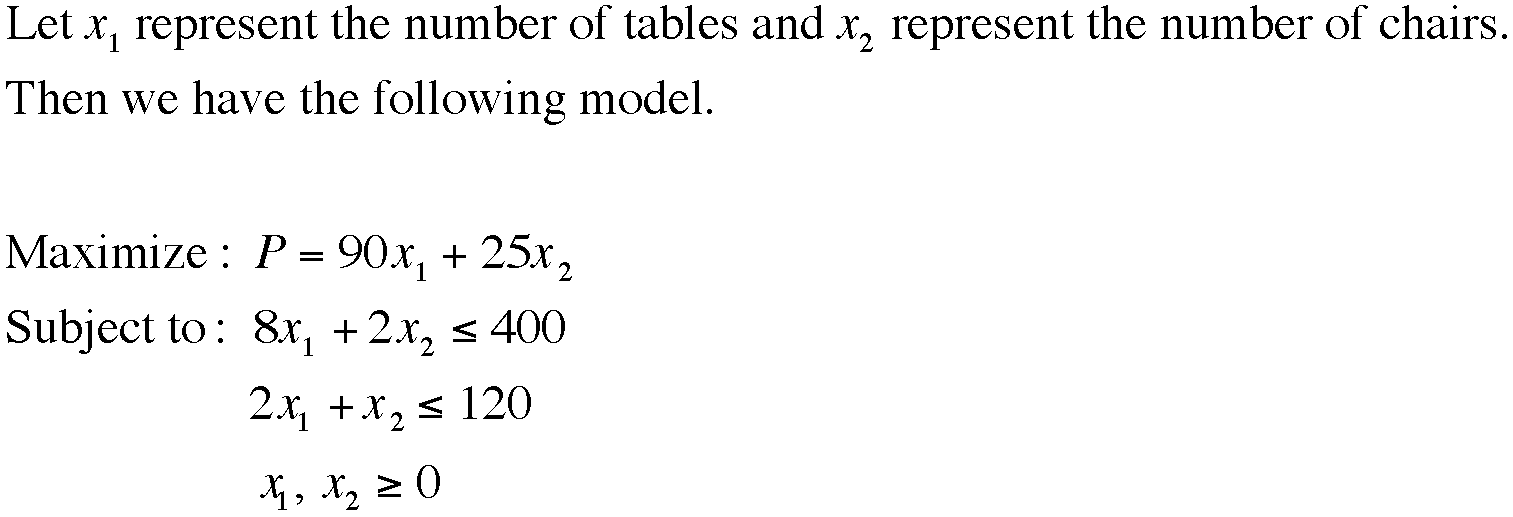
(A) How many tables and chairs should be manufactured each day toorealize a maximum profit? What is the maximum profit?
(B) Discuss the effect on the prductin schedule and the maximum profit if the Marketing Department of the company decides that the number of chairs produced should be at least four timest the number of tables produced.
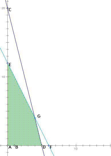
First, we graph the constraint inequalies as equations and identify the feasible region. The feasible region is that area of the graph in which every point satisfies the constraint inequalities. This is the same as solving a set of simultaneous linear inequalities graphically. See below.
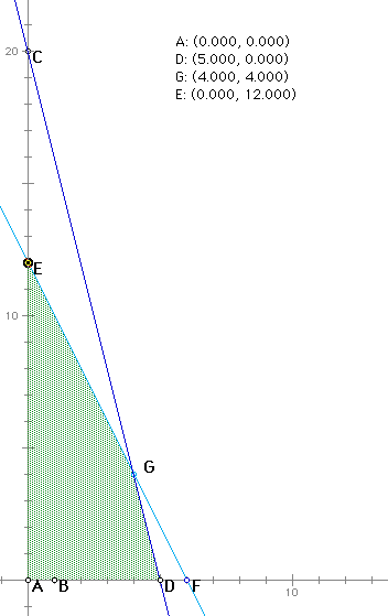
For the purpose of display, the scales have been reduced by a factor of 10. Next, find the coordinates of the corner points of the feasible region using the measure coordinates function of GSP.
Now we solve the objective function for the second independent
variable in terms of the dependent variable and the first independent
variable. When we do we get the following equation. ![]() .
Because of a limitation of GSP, I have scaled the graphs so that
any results must be multiplied by 10 to get the real answer. If
we set P =2500, an graph the result on our previous graph
we get the graph shown below.
.
Because of a limitation of GSP, I have scaled the graphs so that
any results must be multiplied by 10 to get the real answer. If
we set P =2500, an graph the result on our previous graph
we get the graph shown below.
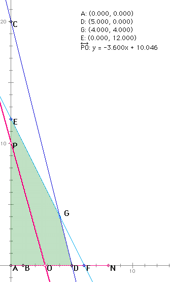
The red line represents the objective function. We have come as close as possible to giving the objective function a value of 2500 as indicated by the constant 10.046 in the equation of the line on the GSP sketch. (we get the value of 2500 by multiplying the constant in the measured equation on the graph by 250.) The value of the constant of the equation of lines parallel to this line multiplied by 250 will always give the value of the objective function for that position of the line. Notice that as we move the red line to the right keeping it parallel, it will first cross point E, then point D, and finaly point G before the line no longer crosses the feasible region. The iterpretation of the line representing the objective function and the feasible region is that, for the portion of the line inside the feasible region, any point on the line is a feasible solution of the LP problem. As we move the line to the right the value of the objective function increases. The value of the objective function is maximum when the line reaches the last possible contact with the feasible region. This is always a corner point or a boundary line. For this reason we have the following theorem
If a linear programming model has a maximum solution, it will be at a corner point of the feasible region.
This theorem takes into account the case of a boundary line because such a line must lie between two corner points of the feasible region.
To show that the maximum solution of this problem is at point G see the sketch below.
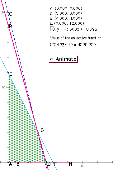
We can see that the last point on the feasible region touched by the objective function is point G. If we place the coordinates of point G into the objective function we get a maximum value of $4600. Notice that the picture above has an animate button. If you have GSP installed on your computer and wish to explore this problem for yourself, click here to go to the GSP sketch used to construct the picture above.
Normally we would not solve a linear programming problem with two independent variables graphically in this manner. We use this technique to show the students how LP works. To solve a problem this small we would do the following. Graph the constraints as above to determine the feasible region. Find the coordinates of the feasible region algebraically by solving the individual systems of equations in two variables associated with each corner point. Make a table of the corner points and the value of the objective function associated with each corner point. Choose the maximum (or minimum) value from the table. The associated table for this problem appears below.

Since the optimal value always occurs at a corner point, there is no need to construct the objective function and move it to determine the optimal value.
Geometer's Sketchpad is a very useful tool for classroom instruction. Linear programming is just one of the ways to use GSP in the classroom. Because of the flexibility of GSP to be able to move and reshape objects and to model functions, you can demonsttate a wide variety of mathematical concepts in a way that enhances learning visually, which is the learning mode of many students. So GSP is not limited to geometry. Linear programming belongs to a field commonly called Management Science or Operations Research. GSP can also be used in instructing calculus. For an example of this see the instructional unit that can be linked to from my EMAT 6690 webpage. Anywhere that mathematical concepts can be illustrated graphically, GSP can be used to enhance instruction. The only thing required is GSP installed on your computer and an active imagination.