A Lesson with string
data on the Excel
Gooyeon Kim and Eduarda Moura
The following data corresponds to the measurements from the
bridge of a guitar to each of the frets:
| Fret # |
Length to
the fret
|
Fret # |
Length to
the fret
|
| 0 |
64.5 |
11 |
34.2 |
| 1 |
60.7 |
12 |
32.3 |
| 2 |
57.4 |
13 |
30.4 |
| 3 |
54.1 |
14 |
28.7 |
| 4 |
51.1 |
15 |
27.1 |
| 5 |
48.3 |
16 |
25.6 |
| 6 |
45.5 |
17 |
24.2 |
| 7 |
43 |
18 |
22.8 |
| 8 |
40.6 |
19 |
21.6 |
| 9 |
38.4 |
20 |
20.4 |
| 10 |
36.3 |
|
|
Students might conjecture that the graph corresponds to a branch
of a parabola or that corresponds to a exponential function. Depending
on the conjecture the teacher might suggest the students to compose
a table of second differences for the parabola or ratios for the
exponential.
Computing the ratios of the values corresponding to 2 successive
frets we get the following sequence:
| Fret# |
Length to Fret |
Ratio |
Fret# |
Length to Fret |
Ratio |
| 0 |
64.5 |
0.941085271 |
11 |
34.2 |
0.944444444 |
| 1 |
60.7 |
0.945634267 |
12 |
32.3 |
0.941176471 |
| 2 |
57.4 |
0.942508711 |
13 |
30.4 |
0.944078947 |
| 3 |
54.1 |
0.944547135 |
14 |
28.7 |
0.944250871 |
| 4 |
51.1 |
0.945205479 |
15 |
27.1 |
0.944649446 |
| 5 |
48.3 |
0.942028986 |
16 |
25.6 |
0.9453125 |
| 6 |
45.5 |
0.945054945 |
17 |
24.2 |
0.94214876 |
| 7 |
43 |
0.944186047 |
18 |
22.8 |
0.947368421 |
| 8 |
40.6 |
0.945812808 |
19 |
21.6 |
0.944444444 |
| 9 |
38.4 |
0.9453125 |
20 |
20.4 |
|
| 10 |
36.3 |
0.94214876 |
|
|
|
The ratio seems to be around the value 0.944. In fact, if we
average the values in the third column we get the value 0.94406996.
The function seems to be exponential with first value 64.5. If
we produce the values of this function in excel we have:
| x |
 |
x |
 |
| 0 |
64.5 |
11 |
34.217766 |
| 1 |
60.888 |
12 |
32.3015711 |
| 2 |
57.478272 |
13 |
30.4926831 |
| 3 |
54.2594888 |
14 |
28.7850929 |
| 4 |
51.2209574 |
15 |
27.1731277 |
| 5 |
48.3525838 |
16 |
25.6514325 |
| 6 |
45.6448391 |
17 |
24.2149523 |
| 7 |
43.0887281 |
18 |
22.858915 |
| 8 |
40.6757593 |
19 |
21.5788157 |
| 9 |
38.3979168 |
20 |
|
| 10 |
36.2476335 |
|
|
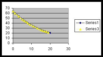
And if we graph simultaneously the original data and the values
given by this new table we can see that the values of the function:

approximates quite well the string data:

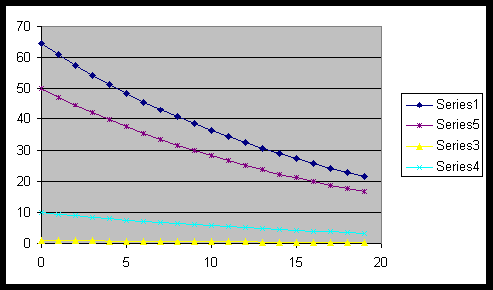
What if we change the length of the open string to 50 or 10
or 1?
|
x |

|

|

|
|
0 |
50 |
1 |
10 |
|
1 |
47.2 |
0.944 |
9.44 |
|
2 |
44.5568 |
0.891136 |
8.91136 |
|
3 |
42.0616192 |
0.84123238 |
8.41232384 |
|
4 |
39.7061685 |
0.79412337 |
7.9412337 |
|
5 |
37.4826231 |
0.74965246 |
7.49652462 |
|
6 |
35.3835962 |
0.70767192 |
7.07671924 |
|
7 |
33.4021148 |
0.6680423 |
6.68042296 |
|
8 |
31.5315964 |
0.63063193 |
6.30631928 |
|
9 |
29.765827 |
0.59531654 |
5.9531654 |
|
10 |
28.0989407 |
0.56197881 |
5.61978813 |
|
11 |
26.5254 |
0.530508 |
5.30508 |
|
12 |
25.0399776 |
0.50079955 |
5.00799552 |
|
13 |
23.6377388 |
0.47275478 |
4.72754777 |
|
14 |
22.3140255 |
0.44628051 |
4.46280509 |
|
15 |
21.06444 |
0.4212888 |
4.21288801 |
|
16 |
19.8848314 |
0.39769663 |
3.97696628 |
|
17 |
18.7712808 |
0.37542562 |
3.75425617 |
|
18 |
17.7200891 |
0.35440178 |
3.54401782 |
|
19 |
16.7277641 |
0.33455528 |
3.34555283 |
Then the graphs are:

The students might want to look at better graphs of the functions
and graph them in another application like the the Graphical Calculator
where the functions can be seen from different zooms.
If the students decide to explore the possibility of the data
fitting a parabola we can ask them to make second differences,
discuss what do the second differences look like if the curve
is a parabola.
The table is:
|
fret |
data |
1st Differences |
2nd Differences |
|
0 |
64.5 |
3.8 |
0.5 |
|
1 |
60.7 |
3.3 |
7.10543E-15 |
|
2 |
57.4 |
3.3 |
0.3 |
|
3 |
54.1 |
3 |
0.2 |
|
4 |
51.1 |
2.8 |
7.10543E-15 |
|
5 |
48.3 |
2.8 |
0.3 |
|
6 |
45.5 |
2.5 |
0.1 |
|
7 |
43 |
2.4 |
0.2 |
|
8 |
40.6 |
2.2 |
0.1 |
|
9 |
38.4 |
2.1 |
7.10543E-15 |
|
10 |
36.3 |
2.1 |
0.2 |
|
11 |
34.2 |
1.9 |
7.10543E-15 |
|
12 |
32.3 |
1.9 |
0.2 |
|
13 |
30.4 |
1.7 |
0.1 |
|
14 |
28.7 |
1.6 |
0.1 |
|
15 |
27.1 |
1.5 |
0.1 |
|
16 |
25.6 |
1.4 |
3.55271E-15 |
|
17 |
24.2 |
1.4 |
0.2 |
|
18 |
22.8 |
1.2 |
-3.55271E-15 |
|
19 |
21.6 |
1.2 |
1.2 |
|
20 |
20.4 |
|
|
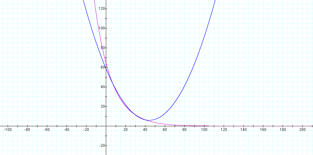
The teacher can also plot the points one by one in the graphical
calculator and ask students to construct the parabola that best
fits the data. Then, to draw the function:

and to discuss again the fitness of the graphs.
The parabola that we found to best fit the data was:

The following is a graph of both functions:

Return to Eduarda's Homepage
