It has now become a fairly standard exercise, with available technology,
to construct graphs to consider equations of the form ![]() . Usually this
is done by overlaying several graphs of
. Usually this
is done by overlaying several graphs of ![]() for different values of a,
b, or c, as the other two are held constant. From these graphs, one can
discover patterns for the roots of various families of parabolas. For example,
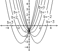
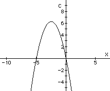
one such family of parabolas can be discovered by letting a=c=1 and varying
b:
for different values of a,
b, or c, as the other two are held constant. From these graphs, one can
discover patterns for the roots of various families of parabolas. For example,
one such family of parabolas can be discovered by letting a=c=1 and varying
b:
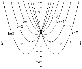
It appears from this family of graphs that the equation![]() has no real roots
when abs(b) < 2, 1 root when abs(b) = 2, and 2 roots when abs(b) <
2.
has no real roots
when abs(b) < 2, 1 root when abs(b) = 2, and 2 roots when abs(b) <
2.
Another way of looking at this relationship is to graph the relation![]() in
the xb coordinate system:
in
the xb coordinate system:
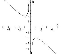
The range of this function represents the values of b which yield real roots of our quadratic equation. Notice this range is the exactly what we concluded from observing the first family of parabolas.
Now consider a similar family of graphs for a=1 and c=-1:
From this graph, it appears that we get two real roots for any value
of b in the equation ![]() . Notice how clear this is from looking at
the relation in the xb plane:
. Notice how clear this is from looking at
the relation in the xb plane:

The range is all real numbers, and each b value "gets used" twice--meaning, for each real value of b there are two real roots to the equation (one positve and one negative).
Now let's vary c while holding a and b constant. By varying the value
of c in the equation ![]() , we get the following family of graphs:
, we get the following family of graphs:
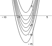
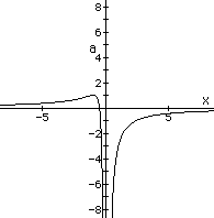
As was expected, since the value of c represents the value of the y-intercept, this family of parabolas is vertically stacked. Now, let's look at this equation in the xc-plane. We can guess, by doing some mental algebra, that this graph will be a parabola:
As before, we can make conclusions as to the nature of the roots of our equations.
Finally, let us vary a, while holding b and c constant. We will graph
the equation ![]() for several different values of a:
for several different values of a:
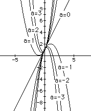
Of note here is the degenerate case when a=0. One wonders how this will appear as we once again look at this graph in the xa-plane:
From this graph we can see, more easily I believe, the nature of the roots for various values of a. We always get two real roots when a<0, we get only one real root when a>0 or a=0, but less than what appears to be 1.
From this exploration, we can see some of the advantages of using several different ways of graphically considering the solutions to quadratic equations. These can be used, as we have done, to study roots; However, this could also be used to study, among numerous other things, graphing, solving literal equations, or solving systems of equations. Students are likely to come up with some interesting and original applications of their own.
Return to Keith Leatham's EMT 668 Home Page