Spreadsheets are very useful tools to use when teaching mathematics. In this write-up, I would like to explore the use of spreadsheets, when displaying the graphs of parametric equations. For the first example, place the initial value of the parameter t in cell A2 and increment t in the A column. I added p/6 to the value in the previous cells. 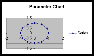In the B column, I put the formula for the x-coordinate, x = cos (t) and in the C column, I put the formula for the y-coordinate, y = sin (t). Below, you will see the worksheet that was created in Excel and the graph to match.

 

t	x = cos (t)	y = sin (t)
0	1	0
0.523599	0.866025	0.5
1.047198	0.5	0.866025
1.570796	6.13E-17	1
2.094395	-0.5	0.866025
2.617994	-0.86603	0.5
3.141593	-1	5.67E-16
3.665191	-0.86603	-0.5
4.18879	-0.5	-0.86603
4.712389	-1.8E-16	-1
5.235988	0.5	-0.86603
5.759587	0.866025	-0.5
6.283185	1	6.43E-16

 

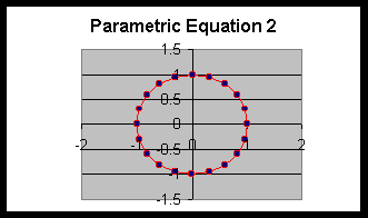
The parametric equation forms a circle. However, I am not pleased with the outcome of the circle. I believe I could graph a better looking circle by plotting more points. My next example, I will have more points and hopefully, I will have a better-looking circle. Below you will see example 2:

 

t	x = cos (t)	y = sin (t)
0	1	0
0.314159265	0.951056516	0.309016994
0.628318531	0.809016994	0.587785252
0.942477796	0.587785252	0.809016994
1.256637061	0.309016994	0.951056516
1.570796327	6.12574E-17	1
1.884955592	-0.30901699	0.951056516
2.199114858	-0.58778525	0.809016994
2.513274123	-0.80901699	0.587785252
2.827433388	-0.95105652	0.309016994
3.141592654	-1	1.22515E-16
3.455751919	-0.95105652	-0.30901699
3.769911184	-0.80901699	-0.58778525
4.08407045	-0.58778525	-0.80901699
4.398229715	-0.30901699	-0.95105652
4.71238898	-1.8377E-16	-1
5.026548246	0.309016994	-0.95105652
5.340707511	0.587785252	-0.80901699
5.654866776	0.809016994	-0.58778525
5.969026042	0.951056516	-0.30901699
6.283185307	1	-2.4503E-16

 
 

Now, the graph resembles a circle. To construct this graph using a spreadsheet, I changed the parameter t values. You do this by changing the formula is the cell A2 and then, copy the cell down the column until you reach the specified range (in this case 0 to 2p).

 

Usually to teach the concepts of parametric equations, you allow the students to find the x and y coordinates manually and graphs the results on graph paper. After 5 or so coordinates, the students become bored with the task. The use of spreadsheets allows students to quickly find the coordinates and graph. Also, students can learn basic spreadsheet skills at the same time.

I would like to explore other parametric equations. What would happen if I added the coefficients a and b to the equations? The resulting equations would look like the following:

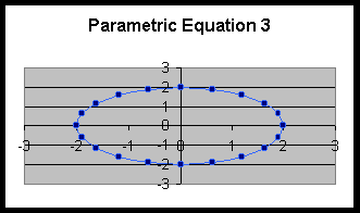
We will try different values of a and b. To do this in Excel, just change the original formula to the desired a and b values and copy the equations down. Here is the result of plugging in 2 and 2 for a and b respectively:

 

t	x = cos (t)	y = sin (t)
0	2	0
0.314159265	1.902113033	0.618033989
0.628318531	1.618033989	1.175570505
0.942477796	1.175570505	1.618033989
1.256637061	0.618033989	1.902113033
1.570796327	1.22515E-16	2
1.884955592	-0.61803399	1.902113033
2.199114858	-1.1755705	1.618033989
2.513274123	-1.61803399	1.175570505
2.827433388	-1.90211303	0.618033989
3.141592654	-2	2.4503E-16
3.455751919	-1.90211303	-0.61803399
3.769911184	-1.61803399	-1.1755705
4.08407045	-1.1755705	-1.61803399
4.398229715	-0.61803399	-1.90211303
4.71238898	-3.6754E-16	-2
5.026548246	0.618033989	-1.90211303
5.340707511	1.175570505	-1.61803399
5.654866776	1.618033989	-1.1755705
5.969026042	1.902113033	-0.61803399
6.283185307	2	-4.9006E-16

 

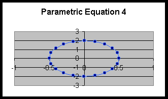
With a few changes, anyone can easily construct a new graph in Excel. Adding the coefficients to the equations, changes the graph to a circle with radius 2. We can do the same for the coefficients 1/2 and 2. The graph is below.

 

t	x = cos (t)	y = sin (t)
0	0.5	0
0.314159265	0.475528258	0.618033989
0.628318531	0.404508497	1.175570505
0.942477796	0.293892626	1.618033989
1.256637061	0.154508497	1.902113033
1.570796327	3.06287E-17	2
1.884955592	-0.1545085	1.902113033
2.199114858	-0.29389263	1.618033989
2.513274123	-0.4045085	1.175570505
2.827433388	-0.47552826	0.618033989
3.141592654	-0.5	2.4503E-16
3.455751919	-0.47552826	-0.61803399
3.769911184	-0.4045085	-1.1755705
4.08407045	-0.29389263	-1.61803399
4.398229715	-0.1545085	-1.90211303
4.71238898	-9.1886E-17	-2
5.026548246	0.154508497	-1.90211303
5.340707511	0.293892626	-1.61803399
5.654866776	0.404508497	-1.1755705
5.969026042	0.475528258	-0.61803399
6.283185307	0.5	-4.9006E-16

How did you expect the graph to look? The graph is no longer a circle, it is now an ellipse. Since we multiplied the x coordinate by 1/2, the ellipse passes through the points (1/2, 0) and (-1/2, 0). The same can be said for the y coefficient, the ellipse passes through the points (0, 2) and (0, -2).

 

There are many other applications of spreadsheets. Teachers can use them to teach most mathematical concepts.