To begin this investigation I feel that it will be beneficial to define the types of equations we will be graphing. Many times in the mathematics curriculum, students graph only using the x and y coordinate system. Parametric equations, however, bring in an independent variable to the situation. This independent variable is called a parameter and in many physical models it is defined as time. For instance the following equations are parametric equations with time as the defining parameter :
If we graph a simple pair of equations
we will need to define the range of t (time).
The following is graphed as t ranges from 0 to 5.
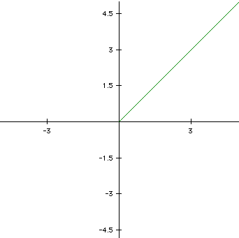
The graph produced is a straight line as time continues. Each coordinate is defined by time. In this graph the coordinates are the same because our equations were equal to t. The starting point of the line began at the origin of the coordinate system when t = 0. If we were to extend the range of t past 5, our line would extend to the number chosen. If we wanted to begin the line at a point other than the origin, we would need to add some constants to our equation.
For example the graph of
looks like
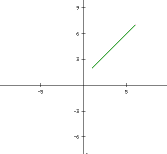
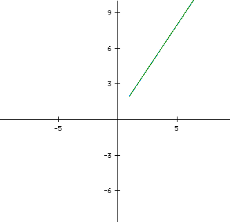
As we have already mentioned the line in the image above is created by the coordinates that are defined by time. That is, when x(t) = 1, y(t) = 1 and so forth. The slope of the line can be defined as simply 1. If we would like to change our slope a coordinate needs to be placed before the parameter of t (time). This will change the parameter from time in intervals of 1, to twice time (2t), thrice time (3t), etc.
The following graph illustrates this concept.
The equations are as follows:

In our investigation, so far, we have graphed only parametric lines. If we would like to produce a curve we need to introduce an exponent. Before we create our equations we need to think about where the exponents need to go. Remember that each coordinate is measured by time. Therefore if we add the same exponent to each graph such as

our coordinates will be defined as time squared. To test our choice, lets assume that time is 2. When we substitute 2 in our equations become
This suggests that our equations will actually produce a line.
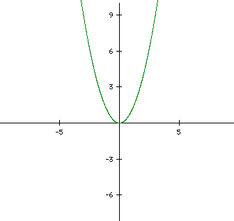
Lets change our equations so that one equation will be defined with t (for our original time) and the other equation as t squared. This will produce a curve.
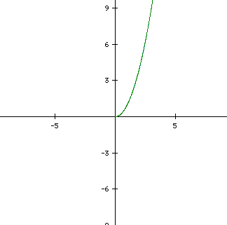
In order to create a curve that "matches" the other side we need to increase the range of time. Our present graph begins when time = 0, therefore, we should extend our range of time into negative values. The following is a graph where time goes from -5 to 5.
Let's advance our equations and investigate

The following graph shows when t ranges from 0 to 1
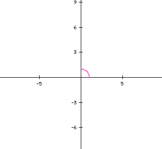
Using this range does not give us enough of an idea what is going on with our equation. It looks as if our curve will be close to a circle. Let's change the range to be from -5 to 5.
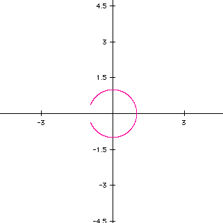
If we increase the range, our graph will continue to look as if the circle will eventually be completed. This, however, is a false assumption. The curve will never meet.
Let's investigate this curve by keeping the range equal to -5 to 5. We will change some of the parameters within the curve.

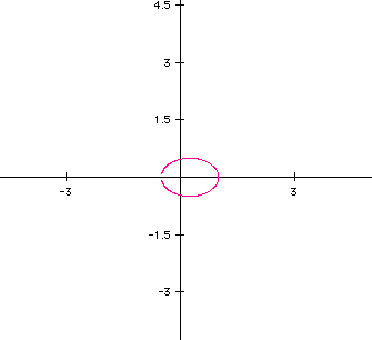
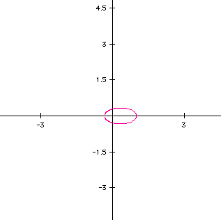
The above equations have been created by increasing the parameter t. The values used, respective to the graphs, are t, 2t, and 3t.
The equations below have the parameters of 1/2t and 1/4t.
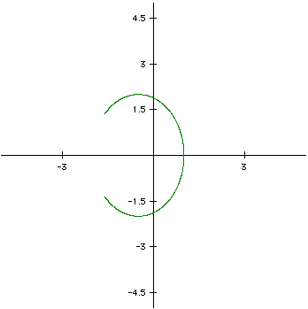
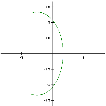
We can clearly see that time affects the graphs. As we increased the time our curve became less and closer to being connected. As we slowed time (through our parameters) we were able to create a larger figure and created a larger gap in the curve.
This investigation is not an in-depth or a complete study of the aforementioned equations. Its purpose was to briefly introduce the concepts of parametric equations. The usefulness of parametric equations can be seen in the physical models of constant motion, where the equation can be defined by only one variable, time.