Suppose we want to determine some information (parameter) about a large population. We cannot easily find the desired information from all the individuals. So, we find a random sample and determine the desired information with repsect to the sample (statistic). The statistic is an estimate of the parameter. But how good is this estimate? According to probability theory, different samples will result in different statistics and thus different estimates of the population. This brings us to the idea of statistical inference.
Statistical inference draws conclusions about a population based on sample data. Statistical inference uses concepts of probability to determine the trustworthiness of our conclusions about the population. This chapter discusses two common methods of inference: confidence intervals and tests of significance. Both of these are based on sampling distributions, i.e., we can determine what happens to the results if we used the method many times.
Note that the statistical inference is most reliable if the sample is a random sample or if data are the results from a randomized experiment.
Note also that Chapter 6 is an oversimplified description of methods. Later chapters will be more rigorous.
If necessary, review the concepts of sampling distributions and the 68–95–99.7 rule. Recall: the law of large numbers states that the sample mean (x-bar) from a large SRS will be relatively close to the population mean (μ) and the Central Limit Theorem states that the distribution of means is normally distributed with a mean the same as the population mean and a standard deviation of σ/sqrt(n). In addition,
Two traditional methods to find the confidence interval (CI) are:
1. use the
68–95–99.7 rule and
2. use the standard normal table.
Luckily,
we can use the TI-83 to find confidence intervals!
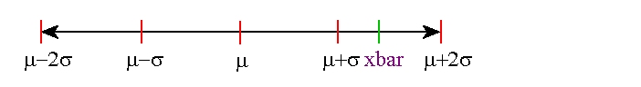
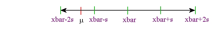
In the long run (i.e., if we calculated the mean of many samples of size n of the population, then 95% of all the samples will have a mean (x-bar) within 2 standard deviations (where the standard deviation is σ/sqrt(n)) of the population mean (μ). This implies that in 95% of all samples, the population mean (μ) is within 2 standard deviations of x-bar!
Here is a picture of what this means:
A level C confidence interval for a parameter consists of:
The confidence interval means: "In a very large number of samples, C% of all the confidence intervals contain the parameter."
From the sampling distribution, if μ is known, then we can standardize x-bar:

where z has N(0, 1) distribution. This is called the
one–sample z statistic.
From this, we get a confidence interval:

where z* is the critical value that can be found:
and where σ is the standard deviation of the population, n is the sample size; and x-bar is the mean of the sample.
The margin of error, m is  .
.
Note that this confidence is correct for normally distributed populations and only approximately correct for large samples of other populations.
Luckily, we can use the TI83 to find the confidence interval and to find the margin of error.
We want high confidence (i.e., our method almost always produces correct estimates) and small margins of error (i.e., a small interval in which we know the parameter exists).
Rearranging the CI formula, we get:

This equation can be used to find the minimum sample size. Don't forget to always round the result up to the next integer.
We can use the TI83 to find n: