EMT 668 Assignment 2

by Jackie Cohen

---

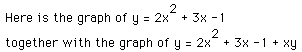
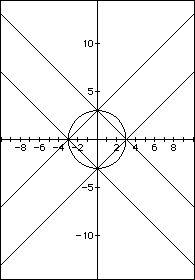
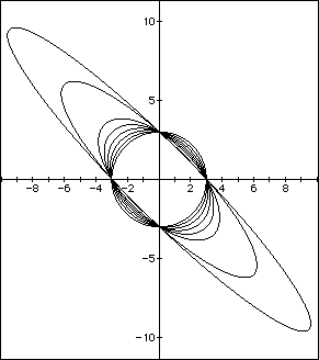
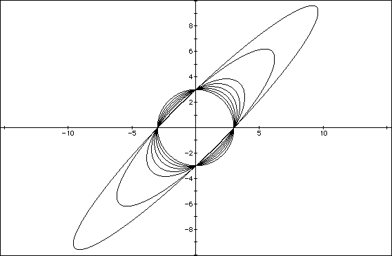
for different values of a, b, and c. Approaching this enterprise in 3 steps, I fixed two of the values for a, b, and c, and varied the third, making at least 5 graphs on the same axes. See the examples below.

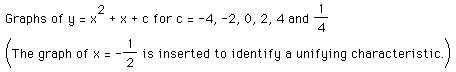
By examining several "families" of such equations for which a and b are constant in each such family, while c varies, we notice that the curves all are alined on a single vertical axis. The value for c always is the y coordinate for the y-intercept since evaluating for x=0 will give y=c as the result. The effects of varyining the coefficients a and b are demonstrated and discussed in the following examples. (This exploration was actually best accomplished on the graphing calculator; the same was true for the two which follow by allowing either a or b to vary and observing the results.)

Note that the line is the graph for the equation when a=0. The graphs for the equations when a< 0 are concave upward and lie completely above the line where a=0. When a>0, they are concave downward and lie completely below that line. Again, each graph interscects the y-axis only at the point (0,c), that is, (0,2) in this example.

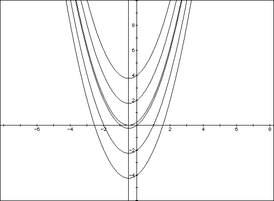
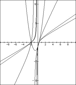
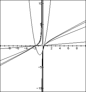
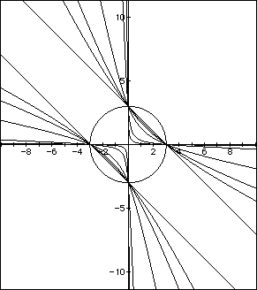
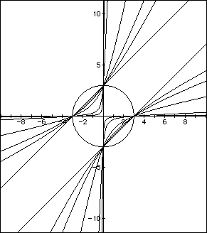
This is , perhaps, the most difficult effect describe; I will explore it further in assignment 3! when b = 0, the curve passes through the y-axis at its vertex. For positive values of b, the curve moves to the right and downward; for negative values of b, to the left and downward. As shown below, for a<0, varying the values of b move the curve up and right for positive values and up and left for negative values.

For demonstrations in a classroom setting, I would prefer to graph each of these families one graph at a time, adding the new graphs to the others until the pattern is perceived. Otherwise, it is difficult to see what the impact of each change is. I would definitlely like to demonstrate these concepts on the graphing calculator. In fact, I would also use the graphing calculator to "back-up" and display several graphs of the following.

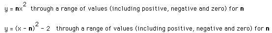
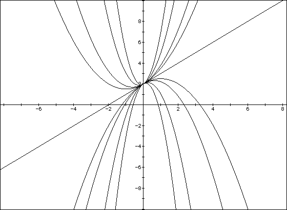
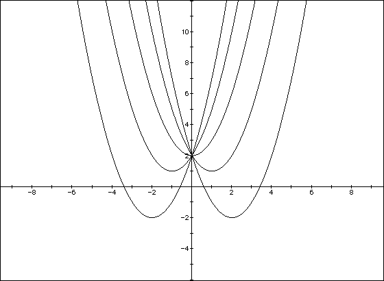
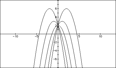
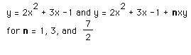
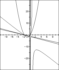
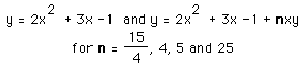
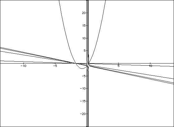
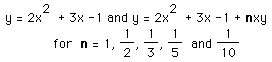
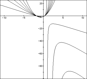
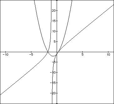
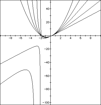
In the first case, we would again observe that when a (now n) is 0, the graph is a horizontal line, when a (now n) is positive the curve is concave upward, and when negative, downward. The larger the coefficient, in absolute value, the tighter the curve; the smaller, the flatter. In the second demonstration, we observe a more predictable way to shift the curves to right and left with positive and negative, respectively, values of n.

Let's explore some other variations of the equation by adding the term xy and then trying different coefficients for the xy term.

Note that both graphs pass through the x and y axes at the same points, as would be expected from the algebra of replacing either x or y with 0. This will remain true for all the variations explored below.

Let's see what happens as the coefficient of the xy term varies.

Note that as the coefficient goes from 1 to 3 1/2, the two "halves" of the curve appear more pointed and the part in the 3rd quadrant appears to approach the y-axis (vertical) with the point close to the y-intercept. In the next graph, the effect of letting the coefficient increase from 3 3/4. (I wonder exactly where the boundary is? Somewhere between 3 1/2 and 3 3/4?)




Note that as the coefficient increases from 3 3/4, again the two "halves" of the curve appear more pointed . But here the curves have flipped to an upper right and lower left part.



Here, as n gets closer to 0 the top part of the curve gets close to the parabloa where n=0 while the bottom part appears to slide away into the 4th quadrant.

Now let's explore what happens when the coefficient of the xy term is negative. The effects are demonstrated below.

Finally, we take a look at another "family" of curves, all built around a familiar one, the circle with center at the origin and radius = 3.

That is, values of n between 0 (where the graph is a circle) and 2 (but not including 2)




These are the graphs of the same equations as above, except that the coefficient, n, of the xy terms are negative instead of positive:

I hope that you have enjoyed this exploration into a small corner of the world of quadratic equations and their graphs.

END OF ASSIGNMENT 2
by Jackie Cohen