The following experiment was conducted using the TI-83 (Texas
Instruments) calculator and the CBL (Calculator-Based Laboratory)
system. We measure the cooling of water with the temperature probe
for the CBL. This data is read every minute and fed into the TI-83
calculator. The calculator, then, graphs the data on the X-Y plane.
Once all data has been read and graphed, we can use the calculator
to find best-fitting curves. We will try a linear, quadratic and
exponential fit. To learn more about the TI calculators and CBL
capabilities and programs, Click
Here.
After uploading the data from the TI to a CPU (using the TI-graph
link), we can plot the time and temperature data on a spreadsheet.
We can graph it on the spreadsheet, as well as graphing the best-fitting
curves. Then we will find the error in our analysis by the least
squares method. This will also be done in the spreadsheet.
| Time (in Seconds) | Temperature (in Celcius) |
| 0 | 89.23 |
| 60 | 89.23 |
| 120 | 85.42 |
| 180 | 82.53 |
| 240 | 79.91 |
| 300 | 77.67 |
| 360 | 75.61 |
| 420 | 73.67 |
| 480 | 71.75 |
| 540 | 70.2 |
| 600 | 68.92 |
| 660 | 67.41 |
| 720 | 66.02 |
| 780 | 64.67 |
| 840 | 63.48 |
| 900 | 62.21 |
| 960 | 61.26 |
| 1020 | 60.05 |
| 1080 | 58.97 |
| 1140 | 58.14 |
| 1200 | 57.26 |
| 1260 | 56.46 |
| 1320 | 55.52 |
| 1380 | 54.68 |
| 1440 | 53.92 |
| 1500 | 53.11 |
| 1560 | 52.37 |
| 1620 | 51.79 |
| 1680 | 50.92 |
| 1740 | 50.43 |
| 1800 | 49.86 |

In each case, X represents time and Y represents temperature,
so we have temperature as a function of time. Also, in each case
we must find the constants, 'a','b' and 'c', that best fit our
data.
Without the calculator, we might guess 'b' will be the initial
temperature of the water, for the first equation, since Y = b
at t=0. Likewise 'c' will be the initial temperature of the water
in the second equation. Then 'a', in the first equation, and 'a'
and 'b', in the second equation will describe how fast the water
is cooling. We could find these values by plugging data into these
equations and solving for 'a', 'b' and 'c', but the caluculator
should be faster and more accurate, since it will consider all
data points.
For the linear fit, the TI-83 chooses, a = -.02 and b = 83.11.
For the quadratic, we have a = 9.33 x E (-6), b = -.04 and c =
89.02.
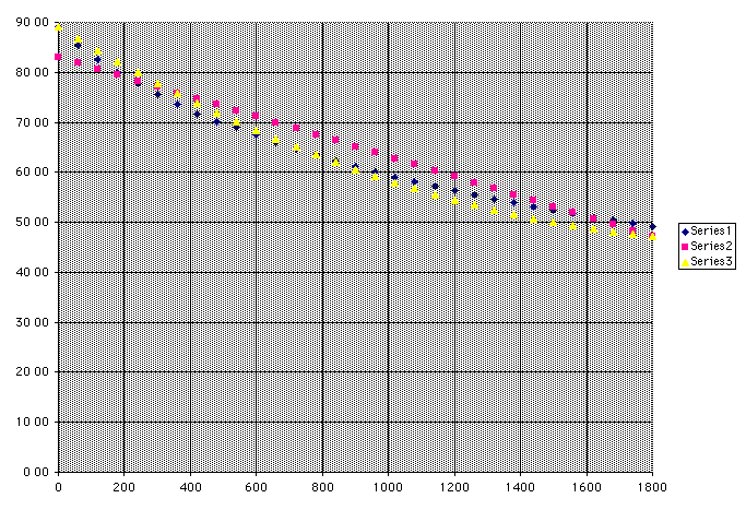
Let's look at these graphs versus our data:

We see the real data in blue. The pink line is the TI's linear
fit. The yellow line is the TI's quadratic fit. Note that the
quadratic fit is pretty convincing. In fact, we can measure just
how convincing it is.
The TI would not give a good exponential regression line because
the 'b' value needed is too close to 1 (the TI approximated this
value to 1 which, you will note, genterates a straight line in
our exponential equation).
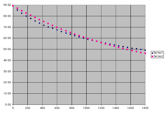
However, by using the least squares method on our spreadsheet,
we can fing a good exponential fit to our data:

We see that the exponential fit is also convincing. We can
use the least squares method to determine which, quadratic or
exponential, is the more fitting fit. Unfortunately, we find that
the quadratic fits the given data a little more accurately (4.09
versus 3.13). This may be because we have an inaccurate room temperate
reading (used in the exponential but not the quatratic equation).
Also, remember that the TI, more nimble than human, calculated
the constants for the quadratic. We calculated the exponential
constants by hand on the spreadsheet.
It is important to realize that the exponential fit is actually
more appropriate. To see this, consider the temperature as hours,
days or years pass. The exponential equation will reveal a tendency
toward room temperature. The quadratic will tend toward a more
Hell-ish one.
To see the spreadsheet with all this data and graphs, Click
Here.
We can use the spreasheet with our exponential equation to predict
the water temperature at unplotted times:
After 45 minutes, we have Temperate = 36.71 degrees Celcius.
After an hour, Temperature = 31.06 degrees Celcius.
After one day, we are at room temperature, as expected.
So, we were able to use the TI and CBL technology to gather data
for us, efficiently and accurately. The TI was also able to offer
some possible regression fits to our data and plot them. Then,
the spreadsheet helped to find a suitable exponential fit with
minimal error. It provided clear graphs for comparisson, and let
us predict temperatures at times not recorded. This is just one
example of how technology can aid in data experiments.