Where does the idea of antiderivative lead? Of what use is it? Equations involving derivatives (differential equations) model many real world problem situations. Understanding antiderivatives and how to compute them is essential to solving such equations.
For you, as a 1st year calculus student, antiderivatives will allow you to (for instance) take the acceleration of an object, and given certain initial conditions, produce formulas for the velocity or position. Therefore if you were taking a Physics course, your calculus knowledge would allow you to produce many formulas that other students must memorize. For a business student, you can (for example) learn how to predict future profit if you know the rate of change of the profit and the present profit.
One of the most important topics for you to study concerning antiderivatives is that of area under a curve. That is, given a function, what is the area bound by that curve and certain other parameters? Let us look at a way of getting at this problem which was first approached by George Riemann, a mathematician of some renown. When we do, we will find ourselves once again faced with infinitesimally small quantities. It is then that we always find ourselves in need of the engine that drives calculus, the limit. Click "rectangles" to begin your study.
Approximating the area under the curve with a sum of rectangles produces an error. Was our figure for the area too large or too small? *How could we reduce the amount of error? Could we allow the rectangles to overhang the curve? Would our figure for the area be too large or too small then?
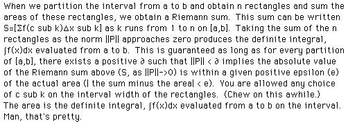
Calculating the approximated area can be done by using the partition P={x sub1,x sub 2,x sub 3,x sub 4,x sub 5} with a rectangle width of delta x and choosing the left-hand endpoints as x values for computing rectangle heights [f(c sub k)]. In other words, we compute Àf(c sub k)delta x sub k as k runs from 1 to n rectangles. In the picture, you see taking left-hand endpoints causes our c sub k's to equal x sub 0 through x sub 4. Delta x sub k's are all .2 since the rectangles are all of the same width. The value of n is 5 rectangles. This is not the only way to set up an approximation. Such sums turn out to be very interesting indeed. For the function in the picture, f(x)=.59x^2, we can write À.59[(c sub k)^2](.2) as k runs from 1 to 5. Click "rectangles" to see the picture again. Mull over what has been said in this paragraph.
If you answered * by saying "increase the number of rectangles used in the approximation", you are correct. Click "hit me" to see this happen.
Increasing the number of rectangles gives a closer approximation to the real area under the curve. The rectangles do not have to be all the same width. The width of the widest rectangle is called the norm, designated || P ||.
How long can we play this game of increasing the number of rectangles and thus decreasing their width? You should know the answer to that if you have studied the limit document on the homepage. If we let the width of the widest rectangle ||P|| go to zero as a limit, all the rectangle widths will go to zero. The question is, what does this mean? It gives us the exact area under the curve, and it will do so from any x=a to x=b on the graph.

Now take a look at the graph of a function f. Study the presentation, and animate to see f. You may use the green show to see the locus. Answer the following questions.......
1. What is the equation of f?
2. What is the area between the curve and the x axis approximated by the rectangles? Measure and see.
3. Calculate the area directly using the integral. How much error is there?
Click "Riemann" to take a look.
The width of the rectangles do not have to be as shown. The choices of c do not have to be fixed just one way. Click "change" and make some adjustments to the rectangles. Adjust the c's anyway you like on their associated subintervals.
Now try your hand at calculating a Riemann sum. Use n=4 rectangles of equal length. Let the function be f(x)=sinx over the interval [-[[pi]],[[pi]]]. Calculate the sum with a choice of c sub k being the left-hand endpoints and then let c sub k be the interval midpoints.
There are many more situations to which one can apply Riemann sums other than area. Basically, if you can slice and dice it (so to speak), you can let the width of the widest slice go to zero (as a limit) and obtain an interesting Riemann sum. If you would like to see another example, click "show me more".
To study more Riemann sums, click "more please"(Old Dominion University)
To return to the homepage, click " loondog".