Lori Pearman
EMT 669
Root - Finding
The zeros of a polynomial f(x) are the solutions of the equation f(x)
= 0. Calculators and computers can be used to find or approximate zeros.
However, before using a computer, it is worth knowing what type of zeros
to expect.
The Fundamental Theorem of Algebra states that if f(x) has positive degree
and complex coefficients, then f(x) has at least one complex zero.
Another important theorem from pre-calculus states that if f(x) is a polynomial
of degree n >0, then there exist n complex numbers C1, C2, . . . ,Cn
such that
f(x) = a(x - C1)(x - C2) . . . (x - Cn)
where 'a' is the leading coefficient of f(x). Each number Ck is a zero
of f(x).
Note that the numbers C1, C2, . . . ,Cn are not necessarily all different.
If a factor x - c occurs m times in the factorization, then c is a zero
of multiplicity m of f(x).
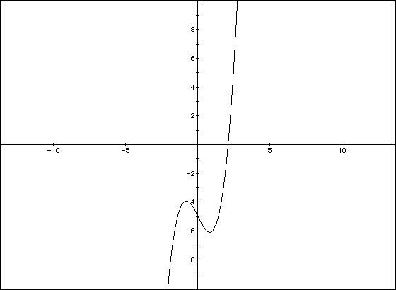
For example, the polynomial f(x) = (x - 2)(x -4)3(x + 3)2 has three distinct
zeros, 2, 4, and -3. The zero 2 has multiplicity 1, the zero 4 has multiplicity
3, and the zero -3 has multiplicity 2. Note that f(x) has degree 6. The
following is a graph of f(x).
Each zero is an x- intercept of the graph of f.
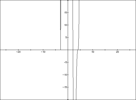
Now let's look at ways in which we can numerically estimate a root of an
equation. Let f(x) = x3-2x-5. Let's graph this function in Algebra Xpresser.
This graph crosses the x- axis between 0 and 5. Let's zoom in on the graph
from x=0 to x=5 to see more accurately where the root is.
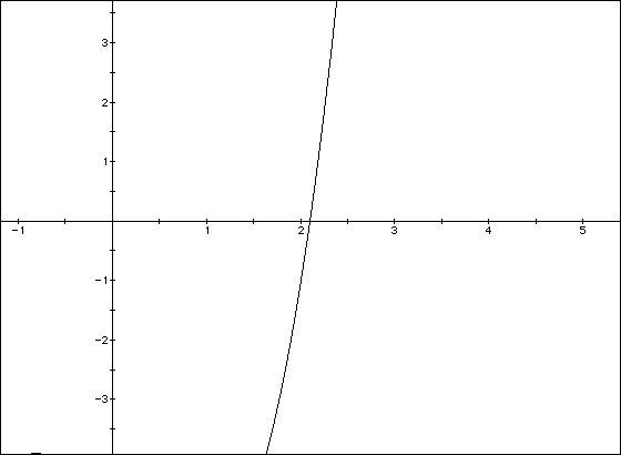
From this graph, we can see that there is a root somewhere between 2 and
2.3. Let's now try to approximate this root using a spread sheet.
     x            f(x)
    2.00         -1.000
    2.01         -0.899
    2.02         -0.798
    2.03         -0.695
    2.04         -0.590
    2.05         -0.485
    2.06         -0.378
    2.07         -0.270
    2.08         -0.161
    2.09         -0.051
    2.10          0.061
    2.11          0.174
    2.12          0.288
    2.13          0.404
    2.14          0.520
    2.15          0.638
    2.16          0.758
    2.17          0.878
    2.18          1.000
    2.19          1.123
    2.20          1.248
    2.21          1.374
    2.22          1.501
    2.23          1.630
    2.24          1.759
    2.25          1.891
    2.26          2.023
    2.27          2.157
    2.28          2.292
    2.29          2.429
    2.30          2.567
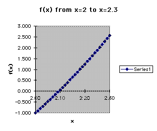
From the above chart, we can see that the root is between x=2.09 and x=2.10.
F(x) is close to zero at these values. Also, the sign of f(2.09) is negative
while the sign of f(2.10) is positive. Let's take a look at the graph of
the chart values.
We can now get a more accurate approximation of the root by using a spread
sheet once again with smaller increments for x=2.09 to x=2.10.
     x            f(x)
   2.090         -0.051
   2.091         -0.040
   2.092         -0.028
   2.093         -0.017
   2.094         -0.006
   2.095          0.005
   2.096          0.016
   2.097          0.027
   2.098          0.039
   2.099          0.050
   2.100          0.061
From the above chart, we can see that the root is between x=2.094 and x=2.095.
We could continue getting better and better approximations of the root by
continuing to look at increments of smaller intervals.
Another way of numerically estimating a root of an equation is by using
the Bisection Method (explained below).
A root occurs when f(x) = 0. If x lies in an interval [a,b] where f(a) is
negative and f(b) is positive, then we can use this information to find
the root.
Take the midpoint of segment ab, and call it `c'. If f(c) is negative, we
know the root lies in the interval [c,b], and if f(c) is positive, we know
the root lies in the interval [a,c].
When we evaluate f(c), we can determine a smaller interval (either [c,b]
or [a,c]) containing the root. Suppose f(c) is negative, and we get the
new interval [c,b]. We can then take the midpoint of this interval and repeat
the same process. The function evaluated at the endpoints of each new interval
should always have opposite signs.
By continuing the process, we are finding smaller and smaller intervals
containing the root. In a sense, we are "closing in" on the root.
Let's look again at the above example. Solve x3 -2x-5 = 0 for a root in
the interval [2,3]. Start with the interval [a,b], where a = 2 and b = 3.
Note that f(a) is negative and f(b) is positive. The midpoint of this interval
is 2.5.
f(2.5) = 5.625, which is positive. Thus, our next interval is [a,c]. Now
take the midpoint of this interval, and call it C2. C2 = 2.25, and f(2.25)
= 1.8906250 which is positive. Our next interval will be [a,C2].
Repeating this process will get you closer and closer to the root since
the interval containing the root is becoming smaller and smaller. The following
chart demonstrates this. (K is the number of iterations.) Each time, f(a)
is negative and f(b) is positive. C is the midpoint of the interval [a,b],
and C will become our new `a' or `b' in the next iteration depending on
the sign of f(c).
     K             a              b             c           f(c)
     1           2.0000000     3.0000000     2.5000000     5.6250000
     2           2.0000000     2.5000000     2.2500000     1.8906250
     3           2.0000000     2.2500000     2.1250000     0.3457031
     4           2.0000000     2.1250000     2.0625000     -0.351318
     5           2.0625000     2.1250000     2.0937500     -0.008942
     6           2.0937500     2.1250000     2.1093750     0.1668358
     7           2.0937500     2.1093750     2.1015625     0.0785623
     8           2.0937500     2.1015625     2.0976563     0.0347143
     9           2.0937500     2.0976563     2.0957032     0.0128626
     10          2.0937500     2.0957032     2.0947266     0.0019548
     11          2.0937500     2.0947266     2.0942383     -0.003495
     12          2.0942383     2.0947266     2.0944825     -0.000770
     13          2.0944682     2.0947266     2.0945974     0.0005125
     14          2.0944682     2.0946045     2.0945364     -0.000169
     15          2.0945435     2.0946045     2.0945740     0.0002513
     16          2.0945435     2.0945740     2.0945588     0.0000811
     17          2.0945435     2.0945587     2.0945511     -0.000004
     18          2.0945511     2.0945587     2.0945549     0.0000382
     19          2.0945511     2.0945549     2.0945530     0.0000169
     20          2.0945511     2.0945530     2.0945521     0.0000063
The interval length decreases from one iteration to the next, "closing
in" on the root which is, correct to 9 decimal places, 2.094551481.
From the computations summarized in the above table, we know that after
20 iterations, the maximum absolute error approximately equals 2.0945530-2.0945521
= 0.0000009.
The bisection method makes no use of the value of f(x) at a particular point
other than to use the sign of f(x) in the selection of an appropriate interval
containing the root. However, it may be helpful to see what the actual value
of f(x) is at particular points. In the above (bisection method) example,
f(2) = -1 and f(3) = 16. From this, we could expect the root to be closer
to x = 2 than to x = 3 (since -1 is closer to 0 than 16 is). So instead
of finding the midpoint of [2,3], let's instead consider a "weighted
average" of 2 and 3. We'll use the regula-falsi method to do
this.
Let [Ak,Bk] be the interval enclosing the root after k-1 iterations. The
regula-falsi method obtains the next approximation x(k) = Ak - (Bk-Ak)f(Ak)/[f(Bk)-f(Ak)].
Call this equation *.
The sign of f(x(k)) may be used to determine whether the root lies in the
interval [Ak,x(k)] or in [x(k),Bk], after which the above equation * may
be applied once again and x(k+1) determined. This may be repeated until
we are satisfied with the approximate root obtained.
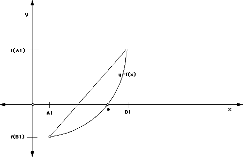
x(k) as given by equation * is the point of intersection of the line joining
Ak, f(Ak)) and (Bk, f(Bk)). During each iteration, the regula-falsi method
approximates the root of f(x) = 0 by replacing f(x) with the secant line
joining the points (a, f(a)) and (b,f(b)), where [a,b] is an interval enclosing
the root. See the below picture. (* is the root we're approximating.)
Unlike the bisection method, the regula-falsi method does not produce an
interval of "small" width enclosing the root. Thus, we need "stopping
criteria" ( to tell us when to stop). In the following example, the
termination criteria is x(n)-x(n-1) < x(n), where > 0 is a prescribed
tolerance.
Let's look again at the problem of solving x3-2x-5 = 0 for a root in the
interval [2,3]. Solve for a root using the regula-falsi method. The below
chart shows the result with = 10-6.
     k             a        b             c             f(c)
     1         2.0000000    3.0000000     2.0588235     -0.390800
     2         2.0588235    3.0000000     2.0812636     -0.147204
     3         2.0812637    3.0000000     2.0896392     -0.054676
     4         2.0896392    3.0000000     2.0927396     -0.020203
     5         2.0927396    3.0000000     2.0938837     -0.007450
     6         2.0938837    3.0000000     2.0943054     -0.002746
     7         2.0943055    3.0000000     2.0944609     -0.001011
     8         2.0944608    3.0000000     2.0945181     -0.000373
     9         2.0945181    3.0000000     2.0945392     -0.000137
     10        2.0945392    3.0000000     2.0945470     -0.000050
     11        2.0945470    3.0000000     2.0945498     -0.000018
     12        2.0945498    3.0000000     2.0945509     -0.000007
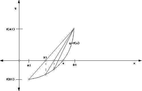
The above picture demonstrates what is happening. Note that this method
may be slow if the graph of f(x) has significant curvature between A1 and
B1.
If the root of an equation is not obvious, it can be estimated in several
different ways. Graphing utilities (such as Algebra Xpresser), spread
sheets (such as in Micosoft Excel), and the methods discussed above
are helpful tools for estimating roots.
References
Asaithambi, N.S. (1995). Numerical Analysis: Theory and Practice.
New York: Saunders College Publishing.
Swokowski, Earl W. (1990) Precalculus:Functions and Graphs. Massachusetts:
pws- Kent Publishing Co.
Return to Lori's EMT 669 Page