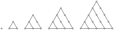
Figure 1. The dynamics of the development of a triangular pattern
The elementary theory of numbers should be one of the very best subjects for early mathematical instruction. It demands very little previous knowledge, its subject matter is tangible and familiar; the processes of reasoning which it employs are simple, general and few, and it is unique among the mathematical sciences in its appeal to natural human curiosity.
G.H.Hardy. (1929). Bulletin of American Mathematical Society, 35, p.818.
The NCTM Curriculum and Evaluation Standards for School Mathematics
(National Council of Teachers of Mathematics, 1989), Everybody
Counts! (National Research Council, 1989), and Reshaping School
Mathematics (Mathematical Sciences Education Board of the National
Research Council, 1990) presented views of the improvement of
mathematics education that give rise to approaches to redefine
mathematics curricula and traditional teaching strategies. This
argues for students becoming more aware of using appropriate technologies,
and more interested in and motivated for learning mathematics
in technology-rich environments. Indeed, technology as a tool
for mathematics investigations brings about opportunities for
new content, new curricula, and new teaching strategies (Lindquist,
Harvey, & Hirsch, 1991).
In the past decade much has been done by mathematics educators
in creating computerized interactive settings aimed at enhancing
visualization as a powerful cognitive support in the learning
of mathematical concepts. Yet, as Eisenberg & Dreyfus (1991)
report, many difficulties with visualization cause student to
gravitate away from visual thinking. Part of the difficulties
might be ascribed to an inadequacy of a single visual representation
of a concept involved, as people seem to have different sensations
of visual information depending on the form in which this information
is presented. Moreover, as suggested by Landesman (1993), sensations
do not necessarily possess propositional content. Attempts to
overcome visualization difficulties have brought about projects
using multirepresentational strategies. These include both combination
of existing computer mathematics systems (Franco, 1991; Dickey,
1993) and designing special purpose learning environments (Schwarz
& Bruckheimer, 1990; Schwarz & Dreyfus, 1993). A project
of Goldenberg (1994) used computer activities to promote an interplay
among geometric, analytic, and algebraic thinking. These approaches
seem to offer promising avenues for contemporary mathematics education;
they stimulate seeking new domains previously not accessible for
multirepresentational educational visualization and the following
pages are about just that.
It may be noted that the use of different forms of computer-generated
visual images in the study of mathematics involves mostly geometry,
algebra, and calculus. But there has been little use of computers
in the teaching and learning of number theory. Yet educational
visualization provided by technology can be integrated into one
of the oldest branches of mathematics. One enjoyable topic in
number theory with little need for prerequisite knowledge is polygonal
(figurate) numbers. The representation of numbers in simple geometric
figures goes back to the arithmetic of the ancients when certain
numbers were noticed to have different characteristics from others.
Before arithmetic was transformed into the theory of numbers people
used simple visual patterns to portray numbers. For example, a
number of objects could be placed like pins in a bowling alley
to form a triangle and in such a way the number becomes triangular.
In much the same way a number of objects can form other regular
polygonal patterns that represent numbers known as square, pentagonal,
hexagonal, etc. All these numbers, as originated from geometry,
are called polygonal numbers. Note that arithmetic and geometry
are the two roots from which has grown the whole of mathematics;
their mutual relation and consequently the more general interrelation
of all mathematical theories has exceptionally great significance.
The approach taken in this article shows that the concepts of
polygonal numbers can be introduced to students not as a final
formalized product, but rather as a result of a gradual elaboration
of a simple geometric construction into an abstract mathematical
model. Besides having historical and aesthetic appeal, integrating
polygonal numbers into curriculum may have an important implication
for pedagogy. Indeed, the awareness of the essential nature of
mathematics and its evolution offers many profound lessons to
anyone trying to be inducted into the field (Guzmán, 1994).
The role of visual strategies in the study of polygonal numbers
has been repeatedly emphasized (Sobel & Maletsky, 1988; Ben-Chaim,
Lappan, & Houang, 1989; Hitt, 1994). In the past, the use
of computers in number theory investigations has not emphasized
visual strategies and required skills in programming languages.
In this article the authors suggest the use of newer software
tools - dynamic geometry, a relation grapher, and a spreadsheet
- to explore, investigate, and discover properties of polygonal
numbers. Mathematical visualization based on these tools provides
a dynamic interplay between geometric, analytical, and numerical
representation of mathematical ideas allowing students to use
this interplay for sense making in mathematics. The replacement
of the process of programming by using a multiple-application
medium is of a great importance to mathematics teaching - it gives
students an opportunity to concentrate their attention on the
subject matter rather than on details of syntax and semantics
of the programming language. It places powerful tools for mathematics
visualization under the control of the students and decreases
an emphasis on authority-centered classroom discourse.
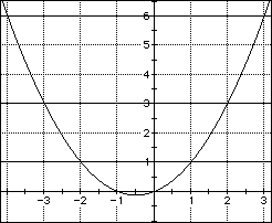
The study of triangular numbers has challenged mathematicians
for centuries. These numbers represent number of dots, discs,
spheres, or similar objects that can be arranged evenly in a triangular
pattern as Figure 1 shows. The dynamics of the development of
a triangular pattern from a set of dots arranged in a triangle
can be visualized with Geometer's Sketchpad (GSP) - a dynamic
software for exploring geometry.
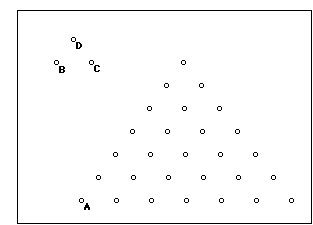
There may be several ways to construct a triangular pattern
by using the GSP's menu-driven transformations such as rotation,
translation, and reflection. Version 2.0 of GSP has the capability
to define transformations based on constructed objects. The first
way may be in using the recursive feature of a script; that is,
to choose an arbitrary point and triangle, and define transformations
based on these objects. The creation of GSP script is described
in Appendix
I, giving a GSP tool called Script RC for generating the
triangular pattern. Figure 2 shows a triangular pattern at 5 levels
of recursion constructed by using Script RC.
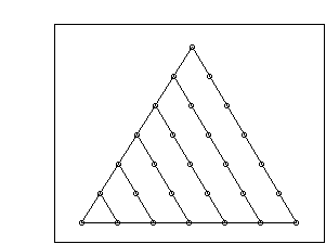
Another way of construction of triangular numbers with GSP
will help students visualize how the triangular pattern evolves
from a set of dots arranged in a triangle. The creation of GSP
script is described in Appendix II, giving a GSP tool called Script
TR for generating the triangular pattern. Choosing three arbitrary
points B, A, and C in a clockwise order (B - the first, A - the
second, and C - the third point), one may play Script TR on these
objects. As a result one can visualize a dynamic construction
of triangular numbers. Figure 3 shows a triangular number of rank
7 presented as a geometric pattern.
One can slightly change the shape of the basic triangle (or
change the distance between points chosen) and construct several
triangular patterns. The activity demonstrates a process of transition
from concrete objects to abstract numbers: different triangles
are connected to the same (triangular) numbers. This is a very
simple but important example of how concepts of arithmetic arose
by way of abstraction, as a result of the generalization of the
practical experience.
Through exploring the triangular pattern of Figure 3, one may
observe that any new side contains one more dot than its precedent.
In other words, by counting dots one can describe the process
of evolving a triangular pattern by the following sequence of
sums of natural numbers
Performing addition results in the sequence of triangular numbers
which can be denoted as t(n).
Depending on how one counts the dots, triangular numbers can be
formulated algebraically in two different ways. As we have already
noted, each step in evolving a triangular pattern from a set of
dots arranged in a triangle increases the number of dots by a
successive natural number, i.e.,
Relation 1 is a recursive definition of triangular numbers
allowing the computation of any triangular number in terms of
a number of the previous rank.
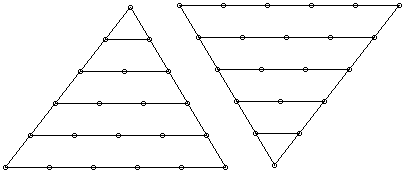
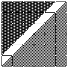
One may count dots, however, not recursively, but directly; that
is, by counting at each step all dots at once. In order to demonstrate
how to do this, let two triangles of rank n (each side contains
n dots) be arranged in the form of a parallelogram (Figure 4).
This parallelogram has n+1 dots at each of n rows. Therefore the
number of dots in the parallelogram is n(n+1), and the number
of dots in the triangle is ![]() , and this is
just the n-th triangular number. So, geometric consideration leads
to another (a closed-form) algebraic formulation of triangular
numbers
, and this is
just the n-th triangular number. So, geometric consideration leads
to another (a closed-form) algebraic formulation of triangular
numbers
One may wonder whether Relations 1 and 2 generate the same
numbers. To make sense of this we suggest using a spreadsheet
- the most widely used application for Macintosh computers. A
spreadsheet makes it possible for students to perform such high-level
mathematics activities as modeling complex situations, investigating
the effects of changing entries on modeling data, discovering
number patterns through visualization, and making and testing
conjectures through numerical evidence. Students often have elementary
skills in operating a spreadsheet and defining functions in cells.
The teacher can exploit this by providing only technical assistance
in the modeling of Relations 1 and 2 on a single template. To
this end in column A positive integral values of n are
defined. In column B triangular numbers are defined through
Relation 1 as follows: cell B1 is entered with the initial
value, cell B2 is entered with the spreadsheet function
=B1+A2 which is then replicated down column B. In
cell C1 the spreadsheet function =(A1*A2)/2 is defined,
computes the first triangular number through Relation 2, and is
replicated down column C. As a result columns B
and C become filled with the same numbers thus confirming
equivalence of Relations 1 and 2 through numerical evidence.
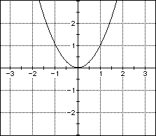
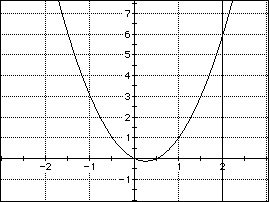
Finally, triangular numbers can be represented analytically.
Throughout the article as a graphing software we employ a dynamic
application Algebra Xpresser (AX) which has the advantage of being
a relation grapher; that is, it allows the graphing of both explicit
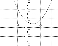
and implicit functions (Goodman, 1993). Due to Relation 2 one
can graph the function y=x(x+1)/2 to get a visual image of triangular
numbers in the form of points with integer coordinates that lie
on a parabola (see Figure 5); that is, positive x-intercepts of
the parabola with level lines y=tn represent a rank of the triangular
number tn. In particular, an opportunity to visualize the existence
of two points on a parabola related to each level line may promote
the idea to consider triangular numbers of a negative rank (Guy,
1994). How could one allow rank to be negative? What is the geometric
interpretation of triangular numbers of a negative rank? This
is only one example of extending and exploring mathematical contexts
with technology tools. Such investigation is part of doing mathematics,
the flavor of teaching and learning mathematics in a dynamic way.
The next remarkable example of polygonal numbers are square numbers.
These numbers represent number of dots, discs, spheres, or similar
objects that can be subsequently arranged by evolving any of these
objects into a square pattern. One can make constructions with
the help of Script
TR. To this end a square has to be constructed first.
Let us denote its vertexes A, B, C, and D cyclically. Now highlight
three of them in the following order: B, A, C and play Script
TR to get half of a square pattern. To complete the square pattern
highlight vertexes D, A, C, in that order, and then play Script
TR. The square pattern has been constructed (Figure 6) and one
can visualize that square numbers are constituted with triangular
numbers. More specifically, any square number is the sum of a
triangular number of the same rank and a triangular number of
the previous rank.
Once a square pattern is constructed, students can visualize the iteration process that generates the dots. This process can be described in the following numerical form
Performing addition leads to the sequence of square numbers
which will be denoted as s(n).
Note that every term of this sequence is the sum of its precedent
and the related odd number. This results in the following recursive
formulation of square numbers
where n is rank of the square number s(n).
Relation 3 can also be constructed through the following geometric
reasoning: each n-th step in evolving a square pattern from a
set of dots arranged in a square adds a gnomon pattern which augments
the number of dots by two times the number of dots on the preceding
side of this square plus one dot, that is, 2(n-1)+1=2n-1.
Obviously, a closed-form formula for square numbers is as follows
What is less obvious, however, is that Relations 3 and 4 determine
the same numbers. As Dubinsky (1991) observed, "mathematics
becomes difficult for students when it concerns topics for which
there do not exist simple physical or visual representations"
(p. 201). Here again a computer can be used to visualize the equivalence
of different formulations through numerical evidence. The power
of visualization provided by a spreadsheet makes this task accessible
for all students at an empirical level through simple comparing
integers in two adjacent columns.
Finally, the use of AX allows a graph of square numbers on the
"rank-side" plane (Figure 7), and it promotes the discussion
about the extension of square numbers to a negative rank. Following
are a few questions which could be asked at that point.
Graphical modeling makes it possible to explore facets of the theory that are not so obvious under the lights of dynamic geometry or a spreadsheet.
The next sequence that arises from evolving a set of dots arranged
into a right polygonal pattern is a sequence of pentagonal
numbers. Here again one can make constructions with the help
of Script TR. To this end a regular pentagon has to be constructed
and label its vertices cyclically, ABCDE. Once pentagon ABCDE
has been constructed, it allows us to start using Script TR as
follows.
Figure 8 shows a pentagonal pattern (pentagonal number of rank 5) constructed by the GSP with Script TR. Likewise in the case of square numbers, one can visualize that pentagonal numbers are constituted with triangular numbers: in particular, this sketch presents a pentagonal number of rank 5 as the sum of a triangular number of rank 5 and two triangular numbers of rank 4.
Observing the sketch and counting the dots within the pattern evolving from a set of dots arranged in a pentagon lead to the following arithmetic description of this pattern:
Performing addition yields the sequence of pentagonal numbers
which will be denoted as p(n).
In order to formulate numbers p(n) in a recursion form one may
note (Figure 8) that each n-th step in evolving a pentagonal pattern
from a set of dots arranged in a pentagon adds a gnomon pattern
that augments the dots' total by one dot plus three times the
number of dots on a side occurred at the (n-1)-th step, that is,
1+3(n-1)=3n-2. This results in the relation
where n is the rank of the pentagonal number p(n).
In order to formulate numbers p(n) in a closed form, note that
any pentagon of rank n is constituted with three triangles - one
triangle of the same rank and two triangles of rank n-1 (Figure
8). Therefore the total number of dots in a pentagon of rank n
equals the number of dots in the triangle of rank n plus two times
number of dots in the triangle of rank n-1. In other words,
The same relation can be constructed through comparing sequences of triangular numbers
and pentagonal numbers
This may result in the observation that due to numerical evidence, any pentagonal number beginning from 5 appears to be the sum of a triangular number of the same rank and two times a triangular number of the previous rank. In other words, Relation 6 holds. To test this finding through numerical evidence one can use a spreadsheet as follows. In columns A, B, and C positive integers n, triangular numbers, and pentagonal numbers are defined respectively. Then cell D2 is entered with the spreadsheet formula =B2+2*B1 which is then replicated all the way down. As a result the sequence of pentagonal numbers occurs in column D thus confirming students' finding through numerical evidence. It may be a challenge for students to use numerical evidence provided by spreadsheet modeling for developing mathematical induction proof of the relation
For more details see Abramovich & Levin (1994).
Finally, one can graph pentagonal numbers on the "rank-side" plane by using AX. That is, to set n=x, p(n)=y, and graph the function
The sketch shown in Figure 9 demonstrates graphically the dependence of a pentagonal number on its rank. Analytical representation of pentagonal numbers allows the raising of the following questions:
These and similar questions stimulate advanced mathematical
thinking and develop skill in exploring complex ideas in a technology-rich
environment.
Let us consider one more special case of polygonal numbers, namely,
hexagonal numbers, which develop from a set of dots arranged in
a hexagon. This pattern can be constructed through the use of
Script TR in much the same way as in the above cases of square
and pentagonal numbers.
To this end a regular hexagon ABCDEF has to be constructed and
label its vertices cyclically, ABCDEF. Once hexagon ABCDEF has
been constructed, its allows us to start using Script TR as follows:
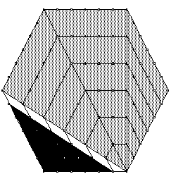
Figure 10 shows hexagonal pattern constructed by GSP with Script
TR. One can visualize that hexagonal numbers are constituted with
triangular numbers: in particular, this sketch presents hexagonal
number of rank 6 as the sum of a triangular number of rank 6 and
three triangular numbers of rank 5.
Observing the sketch of Figure 10 and counting the dots within
the evolving hexagonal pattern result the following arithmetic
description of this pattern
Performing addition yields the sequence of hexagonal numbers
which will be denoted as h(n).
Visualization provided by GSP (Figure 10) suggests two analytic
formulations of hexagonal numbers. A recursive formula
arises from iterative counting of the dots. In order to construct
a closed-form formula for numbers hn one may use a note about
the splitting of any hexagonal number into four triangular numbers,
that is,
Therefore
Here again one can use a spreadsheet to justify through numerical evidence that Relations 7 and 8 generate the same numbers and then use numerical evidence provided by spreadsheet modeling for developing proof of the relation
by mathematical induction.
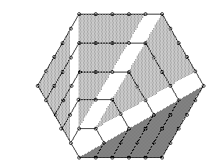
In order to represent hexagonal numbers graphically (Figure 11) students can use AX in graphing the function y = x(2x-1). There are several questions that students can be asked to address at that point.
Of course, a discussion may not be limited to these questions
since more knowledge generates more opportunity for inquiry.
So far we have considered four special cases of polygonal numbers
- triangular, square, pentagonal, and hexagonal. Exploring their
properties in a multiple-application environment makes it possible
to find many common features represented in different settings.
For example, one could observe on the plane of AX that graphs
of Relations 2, 4, 6, and 8 all pass through the point (1,1) and
that this is consistent with the fact provided by GSP that all
polygonal patterns of rank 1 are single dot. Another common feature
could be found through observing these graphs along with the modeling
data of Relations 1, 3, 5, and 7 provided by a spreadsheet: numbers
6, 15, and 28 are triangular and hexagonal at the same time. Furthermore,
the use of GSP made it possible to visualize that any square,
pentagonal, or hexagonal number is the sum of two, three, or four
triangular numbers, respectively. In other words, the sum of triangular
numbers may be a triangular number of a higher rank. All these
examples may motivate students to inquire whether it is possible
to construct an environment for the study of polygonal numbers
of arbitrary side and rank. Generalization will help discover
what is in common and what is not about different polygonal numbers.
The power of visualization provided by GSP makes it possible to
study the general case of polygonal numbers at an empirical, very
intuitive level. This is consistent with an observation made by
Piaget (1966) that "before being able to make a deduction
the subject must observe it empirically in order to accept it
as a true" (p. 232). In this vein, let us consider the GSP
sketch in Figure 10 as a model of polygonal numbers (in this case,
hexagonal numbers) of side m. The number of dots on each
side of a polygon of rank n is exactly n. Denote
P(m,n) as the polygonal number of side m and rank n.
Recursive counting of the dots suggests that the transfer from
n-1 to n in a polygon of side m increases the number of dots by
(m-2)(n-1)+1. This leads to the following recursive definition
of the polygonal number of side m and rank n
subject to the boundary condition
that is, every polygonal number of rank 1 is 1.
By plugging values m=3, 4, 5, and 6 into Relations 9 and 10, one
can verify that Relations 1, 3, 5, and 7 are special cases of
a general recursive definition of polygonal numbers.
One can also count the dots in an m-polygon of rank n
by splitting the polygon into m-2 triangles of the same
rank (Figure 10). Due to Relation 2 each triangle contains ![]() dots and the number of dots on each of m-3 overlapping
sides is n. This way of counting of dots suggests the following
closed-form formula for the polygonal number of side m
and rank
dots and the number of dots on each of m-3 overlapping
sides is n. This way of counting of dots suggests the following
closed-form formula for the polygonal number of side m
and rank
Here again, by plugging values m=3, 4, 5, and 6 into Relation
11 one can justify that Relations 2, 4, 6, and 8 are special cases
of a general closed-form formula for polygonal numbers. Finally,
one may note that due to Relation 11, P(m,1) satisfies Condition
10. The latter may be given the following geometric interpretation:
all polygonal patterns of rank 1 are single dot.
In the previous sections we have discussed the results of analytical
representation of triangular, square, pentagonal, and hexagonal
numbers. It is also possible to explore the general case of polygonal
numbers by graphing Relation 11 with AX. The important advantage
of AX in comparison to other drawing applications is its ability
to graph relations from any two-variable equations. This provides
an opportunity to graph an equation without the need to convert
the latter into a form suitable for "function grapher"
software. So, setting x = n and y = m one can graph Relation 11
on the xy plane for any integer value of its left-hand side. This
would make it possible to discover whether the graph (a level
curve for polygonal numbers) passes through points with integral
coordinates, and if so, every such point represents some polygonal
number whose side and rank are just the coordinates of this point.
The sketch shown in Figure 12 represents the use of AX in the
modeling of the equation
on the "rank-side" plane for C=6, 15, and 28.
The search of points with integral coordinates through which the
level curves pass results in the three pairs of points: (2,6)
and (3,3), (3,6) and (5,3), (4,6) and (7,3). Already mentioned
property of numbers 6, 15, and 28 can be used to interpret this
finding: hexagonal numbers 6, 15, and 28 are also triangular numbers.
Is this true for all hexagonal numbers? Why or why not? This problem
presents an excellent opportunity to explore connections among
different polygonal numbers by visualizing their level curves
in an environment provided by AX.
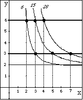
Mathematical visualization of graphical representation of Relation 12 for different values of its right-hand side provokes many profound questions which can stimulate discussion, conjecturing, and computer usage for justifying conjectures through visualization. For example, by changing the scale one may note that each level curve has the same vertical asymptote x=1. In other words, Relation 12 is not defined at the point x=1, though the latter does have a sense in terms of polygonal numbers. Furthermore, each level curve appears to have the same horizontal asymptote x=2, that is, y tends to 2 as x grows large. The following questions arise:
Indeed, speculating on these questions fosters analytic thinking
and promotes dynamic interplay between different representations
of a concept. Moreover, the use of AX in this context allows the
demonstration on a very simple level how analytic thinking can
be integrated into the theory of numbers.
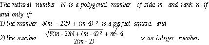
Another benefit that results from Relation 11 deals with a possibility
to construct a test for determining whether integer N is a polygonal
number of side m and rank n. To this end let us multiply the right-hand
side of Relation 11 by 8(m-2) and then add ![]() to
the product. The result is a square because
to
the product. The result is a square because
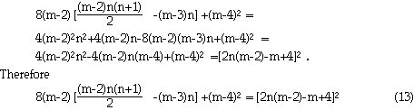
Relation 13 -- known to Diophantus (about 250 A.D.) -- shows that
if integer N is a polygonal number of side m and rank n,
then the expression ![]() should be a perfect square.
This, however, is not sufficient for N to be a polygonal number
- a non-integral value of n may contribute to an integral value
of
should be a perfect square.
This, however, is not sufficient for N to be a polygonal number
- a non-integral value of n may contribute to an integral value
of
Indeed, setting n=7/3 and m=5 in the right-hand side of Relation 14 results in K=13. Resolving Relation 14 with respect to n results the condition providing the integral value for rank n :
This leads to the following criterion which we shall call the
A spreadsheet modeling of polygonal numbers through applying
of the Square Test to natural numbers will be discussed in the
next section.
Hoyles (1994) acknowledges the power of spreadsheet-based intuitive
activities on the construction of polygonal numbers by pointing
at cells by a mouse-pointer and describes a spreadsheet as an
environment "where students generate situated abstractions
of a mathematical nature" (p.174). The spreadsheet, however,
allows students to do more than is generally assigned to it. One
can use the tool to generate these abstractions both in terms
of rank and side, and this provides visualization of polygonal
numbers coordinated at one representation. More specifically,
the computational capacity of a spreadsheet suggests three different
approaches to the modeling of polygonal numbers which include
i) Modeling Relation 9 subject to Condition 10;
ii) Modeling Relation 11;
iii) Applying the Square Test to natural numbers.
A variety of modeling strategies provides representational
plasticity (Kaput, 1992) of a spreadsheet as an interactive medium
allowing a significant enhancement of visual information in the
context of polygonal numbers. In this section we examine ways
in which a multimodeling approach can be put to work.
Approach (i). Note that Relation 9 is a first order difference
equation in two integral variables and that a spreadsheet is capable
for numerical modeling of such equations (Abramovich & Levin,
1994). This can be done through the following simple programming
of a spreadsheet (referred to below as TMG). In column
A and in row 1 positive integers m and n
are defined respectively. In column B beginning from cell
B4 Condition 10 is defined. The spreadsheet function =B4+1+B$1*$A2
is defined in cell C4 and computes the number P(3,2). This
function is replicated to cell U21 by using the Copy and
Paste commands. Note that here and below the $ sign in a spreadsheet
formula designates a coordinate immediately to the right to stay
the same across a template. Therefore, when the above formula
enters into an arbitrarily cell it takes a current value of n
from row 1 in the same column and a current value of m
from column A in the same row. Figure 13 shows spreadsheet
TMG filled with polygonal numbers.
As it has been already mentioned, demonstrated, and verified using
multirepresentational strategies, square, pentagonal, and hexagonal
numbers can be developed from triangular numbers. One can visualize
on a spreadsheet TMG (Figure 13) that this is also true
for polygonal numbers of side more than 6, and therefore to come
up with the following conjecture
In other words, mathematical visualization leads to the discovery of the following theorem attributed to Bachet:
Any polygonal number of side m is the sum of the triangular number of the same rank and m-3 triangular numbers of the previous rank.
Spreadsheet TMG (Figure 13) also allows learners to visualize that polygonal numbers of the same rank constitute arithmetic sequences. More specifically, if P(3,n) is a first term of such sequence then P(3,n-1) is its common difference. Generalization results the following conjecture
In other words,
Any polygonal number of side m equals to the polygonal number of side m-1 and of the same rank plus triangular number of the previous rank.
Students can be encouraged to justify their findings in different
ways -- through numerical evidence (approach (i)) and mathematical
induction (with respect to n). Moreover, as we shall see, Relations
15 and 16 can be visualized with a help of GSP, that is, conjecturing
can be supported by proofs without words.
There are many interesting relations that can be discovered through
exploring numbers in spreadsheet TMG (Figure 13) for example,
to name only one. The challenge for students might be to formulate
the sums of perfect squares and the sums of perfect cubes in terms
of triangular numbers.
Approach (ii). Note that Relation 11 formulates polygonal
numbers in a language of discrete process depending on two integral
variables. Similar to its ability to numerically model equations
of partial differences, a spreadsheet can represent numerically
the right-hand side of Relation 11 for different integral values
of m and n. This has the advantage of modeling polygonal
numbers both of positive and negative rank. The corresponding
spreadsheet is constructed similarly to TMG (Figure 13)
except the function =(B$1/2)*(($A4-2)*B$1-($A4-4)) which
is defined in cell B4 and computes a triangular number
whose rank is indicated in cell B1. Figure 14 shows polygonal
numbers of both positive and negative rank.
Note that even if the teacher has no objective to introduce
the concept of polygonal numbers of negative rank, the students
could arrive at this concept occasionally, erroneously typing
a negative number in cell B1. As a response to that, a
spreadsheet would generate integers arranged into new patterns
so that it might be reasonable for the students to explore polygonal
numbers extended to a negative rank. This is a new way of learning,
when the motivation to study complex ideas stems from activities
of the learner who thereby is aware of the existence of a new
pattern as he or she has generated the pattern.
Approach (iii). Finally, one can model polygonal numbers
through applying the Square Test to natural numbers. As we shall
see below this modeling provides learners with a new arrangement
of polygonal numbers on a spreadsheet template. This, in turn,
makes it possible to visualize new patterns, to explore and discover
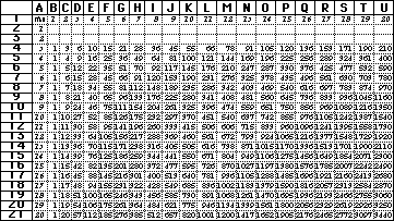
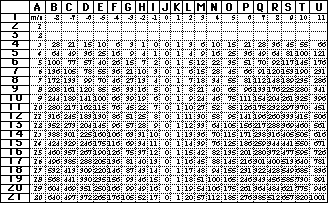
new properties of polygonal numbers. The spreadsheet (referred
to below as TSQ and shown in Figure 15) which implements
the Square Test is programmed as follows. In column A beginning
from cell A2 natural numbers N to which the square test
is applied are defined. In row 1 beginning from cell B1
values of m are defined. In cell B2 the spreadsheet function
=IF(INT(SQRT($A2*8*(B$1-2)+(B$1-4)^2))+
INT((SQRT($A2*8*(B$1-2)+(B$1-4)^2)+(B$1-4))/(2*(B$1-2)))=
SQRT($A2*8*(B$1-2)+(B$1-4)^2)+
(SQRT($A2*8*(B$1-2)+(B$1-4)^2)+
(B$1-4))/(2*(B$1-2)),(SQRT($A2*8*(B$1-2)+
(B$1-4)^2)+(B$1-4))/(2*(B$1-2))," ")
is defined and then replicated across the template. This function tests via the Square Test any positive integer in column A to be a polygonal number of the side displayed in row 1, and if so, a computer fills a cell with the rank of this number, otherwise leaves the cell empty.
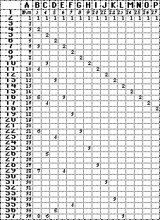
The earlier remark about the advantage of multirepresentational
visual strategies becomes more clear now. Indeed, the environment
provided by spreadsheet TSQ (Figure 15) in comparison with
that of spreadsheet TMG (Figure 13) allows the facilitation
of the discovery of square numbers among triangular numbers, triangular
numbers among hexagonal numbers, and so on. For example, the arrangement
of numbers in Figure 15 clearly shows that 36 is the 8-th triangular,
6-th square, and 3-rd 13-gonal number at the same time. One can
also see that numbers 6, 15 and 28 are triangular and hexagonal
at the same time and this is consistent with the representation
of these numbers through level curves on the "rank-side"
plane of AX. Moreover, changing an entry of cell A2 (or
B1) results in immediate recalculation yielding new data.
This provides the in-depth insight of how the same integers can
represent different geometric patterns. The arrangement of polygonal
numbers on spreadsheet TMG (Figure 13), however, does not
provide a lucid visualization of what is in common about 6, 15,
and 28. On the other hand, spreadsheet TSQ (Figure 15),
being beneficial for many important observations described above,
is not very helpful in the visualizing of arithmetic series and
Bachet's theorem.
The curiosity of students can be highly motivated by the following
demonstrations within spreadsheet TSQ (Figure 15): numbers
21, 2211, 222111, 22221111, ... , as well as numbers 55, 5050,
500500, 50005000, ... , are triangular; numbers 5151, 501501,
50015001, 5000150001, ... , and 45, 4950, 499500, 49995000, ...
, as well as 45, 2415, 224115, 22241115, .... are both triangular
and hexagonal. Moreover, spreadsheet TSQ (Figure 15) displays
the rank of a polygonal number and in such a way students can
visualize, for instance, that 45 (4950, 499500, 49995000) is triangular
number of rank 9 (99, 999, 9999), and hexagonal number of rank
5 (50, 500, 5000). One may then observe that each of these polygonal
numbers is the product of related ranks: 45=9·5; 4950=99·55;
and so on. The following questions arise naturally:
Becoming aware of their ability to discover patterns they never knew before, the students will be highly motivated in answering questions. The teacher can exploit this by encouraging the students to make sense of the above phenomena. The list of questions can be continued:
We believe that speculating on such questions not only develops
skill in making connections among different representations of
a concept, but also provokes guessing and stimulates proving.
Many problems in the theory of numbers are of the following kind:
Express every natural number as a sum of finite number of integers from a given sequence.
Because sums are involved these problems constitute the so-called additive number theory. Mathematics visualization allows students to discover that there are pairs of triangular numbers such that the sum of the numbers in each pair is a triangular number. A natural curiosity may raise the following questions:
To answer these and similar questions students can use a spreadsheet that generates and then sums polygonal numbers of any side given, and tests whether the sum is a polygonal number of the same/different side. A spreadsheet to explore sums of polygonal numbers is programmed as follows. In cell A1 the side of a polygonal number is defined. In row 1 (beginning from cell C1) and column A (beginning from cell A3) positive integers are defined. In cells C2 and B3 the spreadsheet functions
are defined respectively and compute polygonal numbers of the rank indicated, respectively, in cells C1 and A3. These functions are replicated, respectively, along row 2 and column B and display polygonal numbers of the side indicated in cell A1. Finally the spreadsheet function
=IF(AND(C$2>=$B3,INT(SQRT(8*($A$1-2)*(C$2+$B3)+
($A$1-4)^2))=SQRT(8*($A$1-2)*(C$2+$B3)+
($A$1-4)^2),INT((SQRT(8*($A$1-2)*(C$2+$B3)+($A$1-4)^2)+
$A$1-4)/(2*($A$1-2)))=(SQRT(8*($A$1-2)*(C$2+$B3)+
($A$1-4)^2)+$A$1-4)/(2*($A$1-2))),C$2+$B3," ")
is defined in cell C3 and tests whether the sum of two
related polygonal numbers is a polygonal number of the same side.
Computer experiments will lead students to many conjectures about
numbers. And always when any new conjecture occurs the teacher
has the responsibility to encourage students to validate the result
in terms of formal proof rather than through numerical evidence
alone. The latter does not guarantee its existence in the language
of mathematics, but the power of computations suggests cues to
intuition. Moreover, the usage of a computer may lead students
to the forefront of knowledge in number theory explorations. The
teacher should convey his or her respect and admiration toward
hypotheses that result from students curiosity, and thereby boost
students' awareness of themselves as doers of mathematics.
The important theorem of additive number theory that can be conjectured
and validated through special cases is that
Every natural number is
1) either a triangular number, the sum of two such numbers, or at most the sum of three triangular numbers;
2) either a square number, the sum of two such numbers, or at most the sum of four square numbers;
3) either a pentagonal number, the sum of two such numbers, or at most the sum of five pentagonal numbers; and in general,
4) either a polygonal number of side m, or the sum of at most m such numbers.
In spite of the elementary statement of this theorem, stated
by Fermat, its proof - given first by Cauchy about 160 years later
- requires more than elementary means. As Gauss noted, "in
arithmetic the most elegant theorems frequently arise experimentally
as the result of a more or less unexpected stroke of good fortune,
while their proofs lie so deeply embedded in darkness that they
defeat the sharpest inquiries" (cited in Wells, 1988). In
this respect the spreadsheet turns out to be an invaluable medium
for students to do the same mathematics as greatest mathematicians
of the past did. In other words, this setting is conducive to
students' learning of significant mathematical ideas through re-invention
(Freudenthal, 1973; Pólya, 1978).
So far, GSP has served as an environment for developing the concept
of polygonal numbers. Through actual construction of different
polygons and their iterations students learn many powerful ideas
of transformations geometry such as vectors, symmetry, rotation,
reflection, dilation. However, the role of GSP can be significantly
expanded if we consider it as a learning medium allowing demonstration
and geometric interpretation of properties of polygonal numbers
discovered through the use of a spreadsheet. In that way GSP can
be employed to create proofs without words. An example of this
is Bachet's theorem actually presented in a GSP sketch of Figure
10 (the hexagon serves as a model of a polygonal number of side
m). One can visualize that any polygonal number of side m and
of rank n is constituted with a triangular number of the same
rank and m-3 (3 in the case of a hexagonal number) triangular
numbers of the previous rank. The teacher can use color features
of GSP in order to enhance the visualization.
In much the same way the use of GSP provides proof without words
of Relation 16. Indeed, as Figure 16 shows, any polygonal number
of side m and of rank n is constituted with a polygonal number
of the previous side and of the same rank plus triangular number
of the previous rank. It may be exciting activity for students
- to discover properties of polygonal numbers on a spreadsheet
template (or on a plane of AX) and then, in turn, to create proofs
without words with a use of dynamic geometry.
In this article we have demonstrated the usefulness of the multiple-application
medium for the study of polygonal numbers. Although the mathematics
content is not common secondary school curriculum it does not
require any knowledge beyond whole numbers, quadratic functions,
and geometry of regular polygons, and therefore it is relevant
to the 7-12 level.
It should be articulated why the software triple - dynamic geometry,
a relation grapher, and a spreadsheet - has been chosen as a learning
environment for this study. First, the dynamics of an iterative
development of any polygonal pattern from a set of dots arranged
in a regular polygon can be clearly visualized using dynamic geometry
software like GSP which allows to define transformations based
on constructed objects and use these transformations iteratively.
Next, AX extends the capability of function grapher software and
it allows the user to construct level curves for polygonal numbers
without the need to convert their equations into an explicit form.
The availability of level curves provides analytical visualization
of different geometric interpretations of the same numbers. Finally,
a spreadsheet is a generic computing tool allowing numerical representation
of recursively defined concepts, including those expressed by
equations of partial differences. All this makes it possible to
use this software triple as a scaffold of the learning environment
for polygonal numbers.
Several pedagogical changes and benefits occur in a computer-enhanced
environment because the latter makes it possible to treat mathematical
ideas more completely and in greater depth, to discuss many profound
questions which the teacher and students alike may raise naturally
due to the ease and variety of visual representations of ideas.
Many open-ended questions that are dispersed across the article
serve as an extension of basic activities, and they are aimed
at promoting students' advanced mathematical thinking. In this
setting the teacher's intervention into the students' work focuses
on monitoring learning and provoking creative thinking, on bridging
the gap between what students see and what can be actually seen,
on helping to see the general beyond the particular (Hoyles, 1994).
This makes the point clear that seeking an end to authority-centered
classroom does not imply the neglecting of the role of the teacher
in the learning process. On the contrary, the shift of this role
from a giver of knowledge to a mediator and facilitator of students
learning highlights the teacher as an important actor in the process
of students mathematical development.
Another significant implication of a technology-rich classroom
environment is to alleviate intellectual risks felt by students.
Indeed, a computer serves as a reliable partner in helping students
to address teacher's questions. When communicating an answer in
this setting a student is aware of the success, as his or her
argument has been obtained through interaction with software.
In the case when spreadsheet modeling is involved, one proceeds
from numerical calculations, something that mathematical epistemology
considers as the most fundamental method which is both heuristic
and demonstrative (Beth, 1966). Furthermore, the mental freedom
of students serves as another factor which influences the learning
process allowing students not only to seek answers but, better
still, to come up with their own questions thus bringing about
powerful instances of learning. An unusual student inquiry as
occurred through visualization, may unexpectedly touch upon a
new mathematical idea thus yielding the meaningful extension of
the topic discussed.
The flexibility of multirepresentational strategies in the
context of independent or small group explorations accommodates
learners of different abilities. One can easily modify problems
under investigation, and change the degree of the complexity of
the ideas being explored. In this classroom dynamic, the use of
technology is not necessarily a factor that "slows the pace
of instruction" (Harvey & Osborne, 1991, p.83), but on
contrary, it allows to increase the number of questions asked,
augment students' enthusiasm for schooling, and foster their curiosity
and higher-level thinking and reasoning skills. It seems to be
of a great importance for mathematics teaching and learning that
students' involvement in the discussion of complex ideas may occur
occasionally, for example, through "playing" with entries
of a spreadsheet template, zooming on graphs of AX, coloring triangulated
polygons in GSP sketch, and so on.
Finally we argue that multiple-application medium suggested in
this article is not only a means to represent knowledge in more
than one way, but it is also a powerful cognitive support for
learners to move flexibly among different levels that structure
the learning process. According to constructivist approach the
learner reflects on his or her own activity through reconstructing
earlier schemes on a higher level, where they are integrated in
a larger structure. Extending psycho-genetic studies of Piaget
to advanced levels of mathematics, Dubinsky (1991) suggested to
use a computer as a means to induce students into constructive
activities that seem to be useful in acquiring advanced mathematical
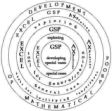
concepts. In the spirit of Dubinsky, the diagram of Figure 17
shows how a multiple-application environment allows in a natural
way the use of coordination, reversal, and generalization as means
for construction of knowledge of polygonal numbers. Indeed, numerical
evidence coordinated with geometric images, and accessibility
of immediate reversal to special cases, provide an ideal medium
for generalization and in some cases could lead learners to the
development of formal proof.
Abramovich, S., & Levin, I. (1994). Microcomputer-based discovering
and testing of combinatorial identities. Journal of Computers
in Mathematics and Science Teaching, 13 (2), 331-353.
Beiler, A.H. (1966). Recreations in the Theory of Numbers.
New York: Dover.
Ben-Chaim, D., Lappan, G., & Houang, R.T. (1989). The role
of visualization in the middle school mathematics curriculum.
Focus on Learning Problems in Mathematics, 11(1),
49-60.
Beth, E.W. (1966). Strict demonstration and heuristic procedures.
In E.W. Beth, & J. Piaget, Mathematical epistemology and
psychology. (W. Mays, Trans.). Dordrecht, The Netherlands:
Reidel.
Dickey, E.M. (1993). The golden ratio: A golden opportunity to
investigate multiple representations of a Problem. Mathematics
Teacher, 86 (7), 554-557.
Dubinsky, E. (1991). Constructive aspects of reflective abstraction
in advanced mathematics. In L.P. Steffe (Ed.), Epistemological
foundations of mathematical experience. New York: Springer
Verlag, 160-202.
Eisenberg, T., & Dreyfus, T. (1991). On the reluctance to
visualize in mathematics. In W. Zimmermann, and S. Cunningham
(Eds.), Visualization in Teaching and Learning Mathematics
(pp. 158-164). Washington, DC: Mathematical Association of America.
Franco, R. di. (1991). Visualization in intermediate analysis
courses in an integrated computer environment. In W. Zimmermann,
and S. Cunningham (Eds.), Visualization in Teaching and Learning
Mathematics (pp. 158-164). Washington, DC: Mathematical Association
of America.
Freudenthal, H. (1973). Mathematics as an Educational Task.
Dordrecht, The Netherlands: Reidel.
Goldenberg, E.P. (1994). Connected geometry: Geometric thinking
in algebra and analysis; analytic and algebraic thinking in geometry.
Paper presented at the Seventh annual international conference
on technology in collegiate mathematics, Walt Disney World Dolphin,
Lake Buenda Vista, Florida.
Goodman, T. (1993). Algebra Xpresser [Technology review]. Mathematics
Teacher, 86 (2), 168.
Guy, R.K. (1994). Every number is expressible as the sum of how
many polygonal numbers. American Mathematical Monthly,
101, 169-172.
Guzmán, M. de. (1994). The origin and evolution of mathematical
theories. In D.F. Robitaille, D.H. Wheeler, and C. Kieran (Eds.),
Selected Lectures from the 7th International Congress on Mathematical
Education (pp. 147-155). Les presses de l'Université
Laval.
Harvey, J.G., & Osborne, A. (1991). A calculator and computer
technologies in mathematics classrooms: A user's guide. In F.
Demana, B.K. Waits, and J. Harvey (Eds.), Proceedings of the
second annual conference on technology in collegiate mathematics:
teaching and learning with technology (pp. 74-86). Reading,
MA: Addison-Wesley.
Hitt, F. (1994). Visualization, anchorage, availability and natural
image: polygonal numbers in computer environments. International
Journal of Mathematical Education in Science and Technology,
25(3), 447-455.
Hoyles, C. (1994). Computer-based microworlds: A radical vision
or a Trojan mouse? In D.F. Robitaille, D.H. Wheeler, and C. Kieran
(Eds.), Selected Lectures from the 7th International Congress
on Mathematical Education (pp. 171-182). Les presses de l'Université
Laval.
Kaput, J. J. (1992). Technology and mathematics education. In
D. A. Grouws (Ed.), Handbook of research on mathematics teaching
and learning (pp. 515-556). New York: Macmillan.
Landesman, C. (1993). The Eye and the Mind. Dordrecht,
The Netherlands: Kluwer.
Lindquist, M.M., Harvey, J., & Hirsch, C. (1991). How mathematics
content courses must change in light of technology and the NCTM
curriculum standards. In F. Demana, B.K. Waits, and J. Harvey
(Eds.), Proceedings of the second annual conference on technology
in collegiate mathematics: teaching and learning with technology
(pp. 20-27). Reading, MA: Addison-Wesley.
Mathematical Sciences Education Board of the National Research
Council. (1990). Reshaping school mathematics: A philosophy
and framework for curriculum. Washington, DC: National Academy
of Sciences.
National Council of Teachers of Mathematics. (1989). Curriculum
and evaluation standards for school mathematics. Reston, Va.:
Author.
National Research Council. (1989). Everybody counts! A report
to the nation on the future of mathematics education. Washington,
DC: National Academy of Sciences.
Piaget, J. (1966). Psychological problems of "pure"
thought. In E.W. Beth, & J. Piaget, Mathematical epistemology
and psychology. (W. Mays, Trans.). Dordrecht, The Netherlands:
Reidel.
Pólya, G. (1978). Guessing and proving. Two-Year College
Mathematics Journal, 9, 21-27.
Schwarz, B., & Bruckheimer, M. (1990). The function concept
with microcomputers: Multiple strategies in problem solving. School
Science and Mathematics, 90(7), 597-614.
Schwarz, B., & Dreyfus, T. (1993). Measuring integration of
information in multirepresentational software. Interactive
Learning Environments, 3(3), 177-198.
Sobel, M.A., & Maletsky, E.M. (1988). Teaching mathematics
(2nd ed.). Englewood Cliffs, NJ: Prentice Hall.
Wells, D. (1988). The Penguin dictionary of curious and interesting
numbers. London: Penguin Books.
1. Construct point A;
2. Construct triangle BCD;
3. Open SCRIPT and click "REC" (start recording).
Following are transformations based on objects chosen in items 1 - 2:
4. Highlight points B and C (in that order), go to TRANSFORM menu and click Mark Vector BÆC.
5. Highlight point A, go to TRANSFORM menu, click TRANSLATE, choose the line "By Marked Vector" and then OK. Denote the new point as E.
6. Highlight points B and D (in that order), go to TRANSFORM menu and click Mark Vector BÆD.
7. Highlight point A, go to TRANSFORM menu, click TRANSLATE, choose the line "By Marked Vector" and then OK. Denote the new point as F.
8. Highlight points E, B, C, D (four objects), go to the SCRIPT, click Loop, then Match, then Loop.
9. Highlight points F, B, C, D (four objects), go to the SCRIPT, click Loop, then Match, then Loop.
10. Click STOP (stop recording information). Highlight all, then copy and paste to a script (call Edit Menu), and save as Script RC.
11. To use Script RC select four points A, B, C, D , go to the Script RC, play the Script, and choose the depth of recursion (which depends on a computer memory capacity).
Return
1. Construct an arbitrary triangle ABC (a triangular number of the second rank).
2. Mark Vector "AÆB" and translate triangle ABC (dots B and C, edges AB and CB) by this vector.
3. Mark vector "AÆC", translate parts of triangle the by this vector and connect dots in order to complete the image of triangular number of the third rank.
4. Repeat this construction to get an image of a triangular number of a chosen rank.
5. Highlight all, then copy and paste to a script (call Edit Menu). Save as Script TR.Return
This paper presents newer software tools - dynamic geometry, a
relation grapher, and a spreadsheet - as an environment for the
study of polygonal numbers through the use of multirepresentational
strategies. The approach is based on developing recursive and
closed formulations of polygonal numbers using computer-generated
geometric patterns. The unique capability of computing and graphing
software involved in the learning environment provides numerical
and analytic representations of discrete concepts depending on
two integral variables. This makes it possible to visualize in
different settings polygonal numbers generalized from special
cases both in terms of rank and side. Advanced mathematical visualization
allows learners to recognize non-trivial patterns among polygonal
numbers invisible within any other medium; to make conjectures
and then, in turn, to justify these conjectures by interpreting
computer-generated numerical evidence, geometric shapes, and graphs.
Even though these may be elementary conjectures their proof often
requires more than elementary means and in these cases computer
applications provide demonstration only. In some cases, however,
mathematical visualization stimulates the development of formal
proof.