

Informally, when we think of one variable depending upon another, we speak of one variable being a function of another. There will often be constraints on the values for any dependent variable, especially when it represents an actual quantity in the real world. The set of possible values for the independent variable is called the domain. Similarly, there are constraints on the values for any dependent variable. The set of possible values for the dependent value is called the range.
In mathematics, we use the term function in a more precise way. One variable y is said to be a function of another variable x if each value of x determines a unique value of y. We call x the independent variable and y the dependent variable. Graphs of functions are traditionally drawn with the independent variable on the horizontal axis and the dependent variable on the vertical axis. Given two linear or first-degree functions, we can allow our students to perform mathematical operations on the functions to discover domains, ranges, and other valuable tools.
First, we'll look at those functions that have no constraints with respect to the domain and range. Thus, the domain and range of these types of functions include all real numbers.
The Sum of two Functions:
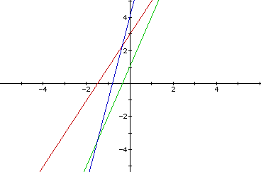
For example, let f(x) = 2x + 3 (red) and g(x) = 3x + 1 (green). Note that both functions have both a positive slope and y-intercept. If we graph these two slopes along with h(x) = f(x) + g(x) (blue), we see that all three slopes are linear. Additionally, the slopes and y-intercepts are merely the sum of the two slopes and y-intercepts, respectively, in the original functions. Clearly, this is the same for adding any two linear functions. When graphing the sum of two linear functions, the domain and range include all real numbers.
Composite Functions:
Often, two functions are combined, not by an algebraic operation such as addition, multiplication, or division, but by letting the second function act on values of the first function. The result is a composite function. Thus, given any two functions f and g, the composite function f o g is the result of the function f acting on values of the function g. That is, (f o g )(x) = f(g(x)).
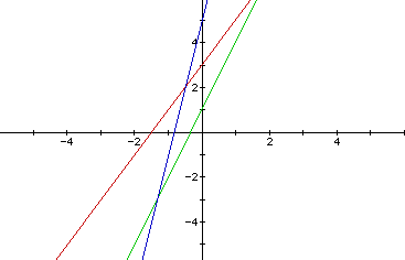
Consider, again, the functions f(x) = 2x + 3, g(x) = 3x + 1. Now, let h(x) = f(g(x) as graphed below. Note that the composition of two linear functions produces a linear function, which can be discovered graphically as depicted here. Thus, as indicated by the graphs below, the domain and range for the composition of linear functions include all real numbers.
Now, we'll consider those functions that have limitations with respect to the range. To increase students' understanding of such limitations, a graphical representation should be discussed as described below.
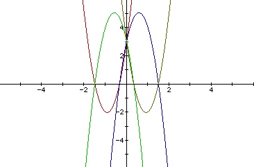
From the following graphs, we can hypothesize that if the product of two functions are graphed, the result is always a parabola. For instance, let f(x) = 2x + 3, g(x) = 3x + 1, p(x) = -2x + 3, and q(x) = -3x + 1. Now, Figure 3 illustrates, let h1(x) = f(x)*g(x) (red), h2(x) = f(x)*q(x) (green), h3(x) = p(x)*g(x) (blue), and h4(x) = p(x)*q(x) (brown). Note that when two positive-slope and two negative-slope functions are multiplied, the result is an upward parabola. In contrast, when a negative-slope and a positive-slope function are multiplied, the result is a downward parabola. This is because, in the standard form of a parabola, a function f(x) = ax2 + bx + c is a downward parabola when "a" is negative, and upward when "a" is positive. The domain of the product of two linear functions includes all real numbers. The range of this type of product is either greater-than-or-equal-to the vertex if the parabola is an upward parabola (the "a" coefficient is positive), or less-than-or-equal-to the vertex if the parabola is a downward parabola (the "a" coefficient is negative). This can be discovered through graphing various products of functions as illustrated below.
This discussion may be also include the quadratic equation, as the limit of the range is the value of y, which when substituted into a quadratic equation, makes the discriminant less than zero, which in turn, produces zeros of the function that are complex numbers.
For instance, h2(x) = f(x)*q(x) = (2x + 3)(-3x + 1). Here, the vertex is at (-7/12, 121/24) which equals approximately (-.583, 5.04). The graph is a downward parabola, so the range is restricted to less-than-or-equal-to 121/24 or approximately 5.04. Substituting a value greater than 5.04 for y=h2(x) produces a discriminant less than zero. This graphical representation should produce several more ideas of how to combine graphing parabolas with introducing limitations with respect to ranges of parabolas and the quadratic equation.
The Quotient of two Functions:
An interesting phenomenon occurs when finding the quotient of two linear functions. If the denominator is zero in a rational number, the number is undefined. Thus, if the denominator of a function contains a variable, the function is undefined when a number exists such that when it is substituted for the variable, it makes the denominator zero. This leads us to a discussion of asymptotes.
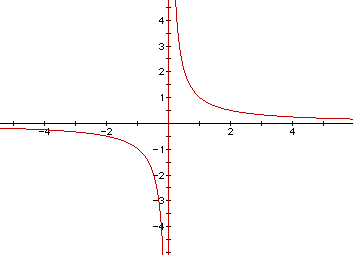
The graph of y = 1/x is shown below in Figure 4. The y-axis, with the equation x = 0, is called the vertical asymptote of the graph. The x-axis, with the equation y = 0, is called the horizontal asymptote. The distance between the graph and its asymptotes approaches zero; that is, the graph gets closer and closer to its asymptotes without ever reaching them.
To obtain a better understanding of the quotient of functions and asymptotes, graph the quotient of the following functions as we did previously with the product of the functions. Let f(x) = 2x + 3, g(x) = 3x + 1, p(x) = -2x + 3, and q(x) = -3x + 1. Now, let h1(x) = f(x)/g(x), h2(x) = f(x)/q(x), h3(x) = p(x)/g(x), and h4(x) = p(x)/q(x). The quotients of the functions are graphed separately to be able to depicted the asymptotes as illustrated.
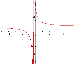
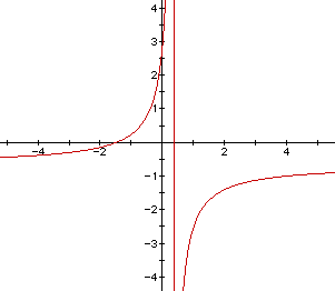
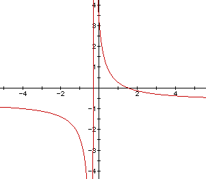

Note that h1(x) has a vertical asymptote of -1/3 and a horizontal asymptote of 2/3. Also note that the graphs of h2(x), h3(x), and h4(x) have vertical asymptotes of 1/3, -1/3, and 1/3 and horizontal asymptotes of -2/3, -2/3, and 2/3, respectively.
From these observations, we can conclude the following rules are when graphing rational algebraic (quotient) functions:
Vertical Asymptotes: If "a" is a value for which the function is not defined, then x = a is a vertical asymptote. This occurs when a value is substituted for a variable which makes the denominator of a function equal to zero.
Horizontal asymptotes: Consider the following function:

Three possible conditions determine a horizontal asymptote:
* If n = m, then y = b/c is a horizontal asymptote.
* If n < m, then y = 0 is a horizontal asymptote.
* If n > m, then there is no horizontal asymptote.
Therefore, the domain of the quotient of two linear functions includes all real numbers except those that, when substituted in for the variable in the denominator, make the denominator zero. These values are also the values that form the equations for the vertical asymptotes. The range can be found by using the above rules depicting horizontal asymptotes.
As illustrated in all of the graphical representations of function above, students who are provided graphical representations my learn the concepts of asymptotes, limits, and constraints of functions better than just merely memorizing rules. Thus, a visual image may be more beneficial when introducing such important mathematical concepts.