

Plotting Points on a Cartesian Plane - A Review
In lesson 1, we briefly mentioned the concept of a coordinate. A coordinate is a numerical value associated with a point on the Cartesian Plane. Basically, a Cartesian Plane is a plane that has two axes at right angles to each other as shown below. The Cartesian Plane is actually a grid (like grid paper) that extends into infinity in four (4) directions. The plane extends up, left, right, and down to infinity (or negative infinity) in all directions. For convenience purposes, the axes are usually drawn in the middle of the plane as it appears on the graph paper. The horizontal axis is always the x-axis, while the vertical axis is always the y-axis. Where the axes intersect is called the origin. The origin serves as the starting point for plotting any coordinate on the Cartesian Plane.
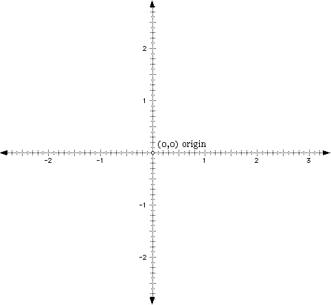
To plot a point on the plane, you must have corresponding x- and y-values to determine where to plot the point. For instance, if you only knew that you were to move right two units and not how far up or down, you would only have half of the information necessary to plot the point. To plot a point, start at the origin and move in across the x-axis, the amount of spaces as indicated. Note that moving left from the origin takes you into the negative integers, whereas to the right of the origin includes the positive integers. For example, if the directions told you to that the x-value of the coordinate was 5, you would start at the origin and move right 5 units (and then up or down on the y-axis as indicated). On the other hand, if the directions told you that the x-coordinate was -6, you would again start at the origin, but this time, you would move to the left 6 units (and then, again, up or down on the y-axis as indicated).
The y-value of the coordinate will either indicate to move up or down on the y-axis. A positive value for the y-value means to move up the y axis (after first moving across the x-axis for the specificied number of units), while a negative y-value means to move down the y-axis (again, after moving across the x-axis, either left or right).
Since space and time are always valuable, people devised ways of making the directions of plotting points condensed. Instead of a long drawn-out explanation that indicates first move left from the origin 5 units on the x-axis (which is the negative direction for the x-axis), then move up 7 units on the y-axis, it is simply written as (-5, 7). Notice that the first number listed correlates with the movement on the x-axis, while the second number correlates with the y-axis as indicated below in the illustration. What a wonderful idea to put coordinates in alphabetical order (x, y)! Note: Don't confuse the coordinate (-5, 7) with interval notation that would represent the domain of a function spanning from -5 to 7, but not including the two endpoints.
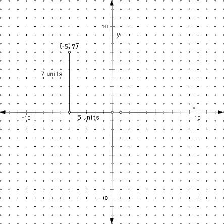
Plot the coordinates: (1, 3); (-2, 4); (-6, -2), (3, -5), (0, 0), (4, 0), (-6, 0), (0, 1) and (0, -5) on your own graph paper the click here to check your answers. This is a very important concept, so make sure that you understand how to plot points on a graph.
Slopes
In Lesson 1 (Functions) we talked about substituting values (we usually used x as the independent variable) into a function and obtaining values for the dependent variable (usually y).
In most of the examples from Lesson 1, the graph was in the form f(x) = ax or f(x) = ax + b. The function that represented f(x) = ax was the gasoline example where "a" was price of gas ($0.80). From this function, we discovered what f(x) would be after picking (substituting) various values of x. So, our function was: f(x) = 0.80x. The function that represented f(x) = ax + b was the first example, f(x) = 5x + 10 and the second example that we graphed, y = x + 2. In the first example, a = 5 and b = 10 in the general for y = ax + b, while in the second example, x = 1 and b = 2.
If you plotted the values of x carefully on each graph, you should have obtained a straight line. Let's go back to the function f(x) = x + 2.
Note, like before that we have a straight line. The line "goes up" from the lower left corner of the graph to the upper right of the graph at a constant rate as all lines do. If a line "goes uleft p" at a constant rate, then it should be clear that the slope of the line is constant. If the slope of a line was not constant, the line would "zig zag" on the from the lower end of the graph to the upper right end.
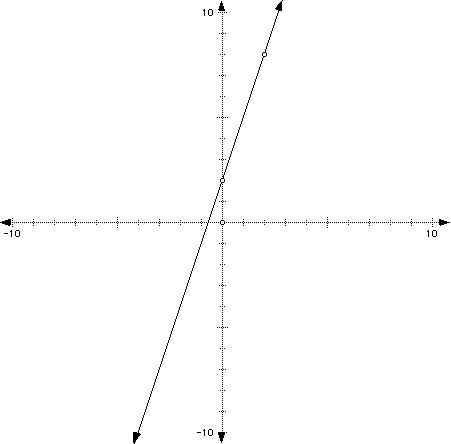
An example of slope
Let's practice graphing another function, f(x) = 3x + 1 on the interval [-4, 4]. We've said before that if we pick values for x and substitute them inot our function, we will corresponding (unique) values for y or f(x) in this case. This means that the point (x, y) that are the actual values of x and y from your substituting and solving would be on the line f(x) = 3x + 1. So, just say we wanted to find a point on this function. Let's pick a value for x to substitute in for x in our function. I'll pick x = 1. Why? Because 1 is a small number to work with and it's pretty friendly. I could have substituted 1,000,000 in for x, but my x-axis would have had to go out 1,000,000 units! If I pick 1 to substitute in for x, I will get f(1) = 3(1) + 1, so f(1) = 4. That means when x = 1, f(x) or y = 1. Therefore, this means that the point (1, 4) is on our line. We could plot the point (1, 4) and know that our line goes through that point. So, let's pick some other numbers to substitute in for x and find their corresponding values of y and plot the points (coordinates) that we get. Since our domain is the interval [-4, 4], we'll pick values of x between (and including) -4 to 4. You really only need to plot two points to make a line, but the more points you plot, the more accurate you can be with respect to graphing the equation. Also note that you can use any values of x between (and including) -4 and 4, however, we suggest to use the most friendly points (so, maybe no fractions or decimals at this time).
|
|
|
f(x) or y-value |
|
|
|
f(-4) = 3(-4) + 1 = -12 + 1 = -11 |
|
|
|
|
f(-3) = 3(-3) + 1 = -9 + 1 = -8 |
|
|
|
|
f(-2) = 3(-2) + 1 = -6 + 1 = -5 |
|
|
|
|
f(-1) = 3(-1) + 1 = -3 + 1 = -2 |
|
|
|
|
f(0) = 3(0) + 1 = 0 + 1 = 1 |
|
|
|
|
f(1) = 3(1) + 1 = 3 + 1 = 4 |
|
|
|
|
f(2) = 3(2) + 1 = 6 + 1 = 7 |
|
|
|
|
f(3) = 3(3) + 1 = 9 + 1 = 10 |
|
|
|
|
f(4) = 3(4) + 1 = 12 + 1 = 13 |
|
|
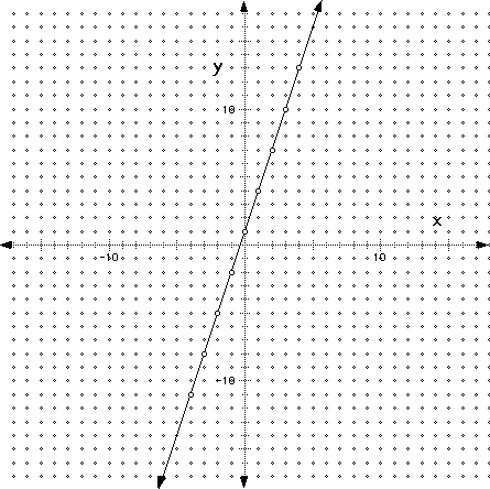
Now, let's plot the last column of the table which represents the values of some of the coordinates on the line. It's important to realize that we picked these values of x just for convenience purposes. We could have pick x = -7, 3, 4, and 17 if we wanted to, found the corresponding values of y, and plotted those coordinates on the graph. You can pick any values that you want for x, and as long as you perform the mathematical operations correctly, and find the correct values for y, the final coordinates (the points in the last column of the table) will make a straight line on a graph.
Let's plot the last column and see if we get a straight line.
Before we proceed with slope, let's take just a few minutes to review the domain and range from lesson 1:
Are there any restrictions on the domain? Remember the restrictions
that we talked about so far are only those that include square
roots and fractions. For example, we cannot take the square root
of a negative number, so if we have a function, we must be careful
not to substitute values of x into the function that would cause
us to take the square root of a negative number. Also, with fractions,
we can never divide by zero, so we must be sure that our domain
does not include numbers that when substituting them into a function
that has a fraction in it that we end up with zero in the denominator.
However, our function is a straight line and does not have any
restrictions on the domain. Also, if we substituted a HUGE number
in for x, to calculate y, we would take that HUGE number, multiply
it by 3 and add 1. If we took a HUGE neagtive number, like -1,000,000
and substituted it in for x, to get y, we would multiply -1,000,000
by 3 to get -3,000,000 and add 1 to get -3,000,001. So, for very
large or very small values of x in this function, we get corresponding
large or small values of y. Notice the arrows on the graph, those
arrows indicate what we just said. This is a good example of showing
that the domain and range both run from negative infinity
to infinity, or ![]() .
.
Now let's proceed with the concept of the slope of a line:
Looking carefully at our graph above, we can determine that the slope is constant throughout the function. Therefore, it doesn't "zigzag" up and down. From the table above, notice that when we proceed from one value of x to the next (i.e., from -3 to -2 or from 0 to 1), the y-value increases 3 units.
Since the y-axis is the vertical axis, the change in the y-axis is also referred to as the rise. This definition should be taken literally, for instance, rise simply means to "go up" and when we plot something on the y-axis, we "go up," or "go up negatively" which really means "fall." Conversely, when you move along the x-axis, you can "run your pencil" across the x-axis. So, another name for the x-axis is the "run". Like the "rise" definition, treat the "run" definition literally. If you were running in a race, surely you would want to run on horizontal ground and not run vertically!
Since we can see that for every 3 units that we move up on the y-axis, we move over one unit on the x-axis, the slope must have something to do with the change in the y- and x-values. You should be able to tell this from the table, too. As stated previously, there is a constant change (adding 3) as we proceed through the values on the table. So, here it is... the fomal definition (one of them) of the slope of a line. Simplify defined, the slope, which is written as "m" for shorthand, is:

Now, what exactly does a change in a variable mean? Let's take an example of a change in temperature. If the temperature has risen from 50 degrees to 60 degrees, how much did it rise? Well, clearly in increased 10 degrees. Formally, we can compute the change of temperature by taking the last temperature (last meaning at a later time than the first temperature) minus the first temperature. So, if we take 60 degrees minus 50 degrees, we get a 10-degree change. Stating this another way, anytime you want to obtain the change in a variable, you can subtract the last variable from the first variable. If this subtraction results in a negative number, the change is a decrease in amount.
Normally when we're working with the change of variables, we have plotted points of a function on a line and are determining the slope between two points. So, let's call two points on a line (x1, y1,) and (x2, y2). The subscript "1" and "2" are there just to tell the difference between the two points. For example, if we wanted to find the slope of the line between the points (2, 3) and (4, 6), and I asked you to identify the "y-value", you could give me two possible answers, namely 3 or 6. However, if I said give me the y-value in the first coordinate (called y1), you would hopefully say 3.
Since the formal definition of the slope is defined as:

Algebraically, we can write this as:

Now, let's pick two points on our line, say (0, 1) and (3, 10) and make sure that we get m = 3 algebraically, since we already know that the slope of the line is 3 in our example, f(x) = 3x+ 1. So, if we calculated the slope using the slope formula above, we would get:

Positive and Negative Slopes of a Line
The aspect of the slope in a function is of utmost importance in everyday situations. The stock market is a good example of how people use slopes. For instance, after completing the tutorial below, you should recognize that going diagonally "up and right" from one point to another produces a positive slope. On the other hand, going diagonally "down and right" from one point to another produces a negative slope. Think of this example: If you are walking and you are going uphill, when you first start-off you are at one point. If you stop 10 seconds later, you are at another point and you have gone uphill. So, you have traveled up a positive slope. Now, if you walk down hill from one point to another point, you are obviously traveling down hill so you are walking on a negative slope. Just be sure that when using this analogy on a piece of paper, you start from the left-hand side of the paper and move right across the graph, just as you would read.
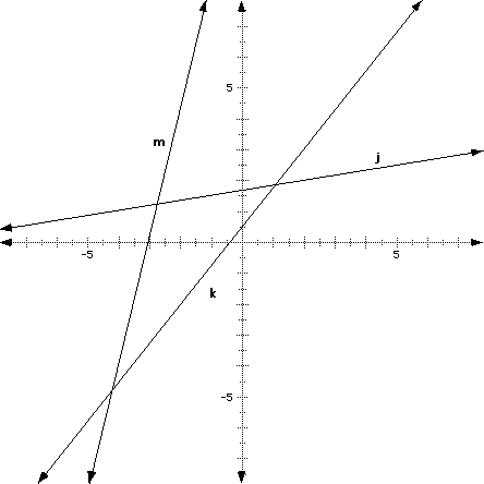
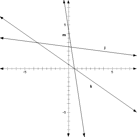
Sometimes the slope equation is a little tricky because of the negative signs already in the formula. However, if you plot the points given, you should be able to tell graphically whether the formula should produce a positive or negative slope algebraically.
For example, find the slope of the line between the points (-4, 3) and (1, 5).
We get the following illustration when we plot the points (-4, 3) and (1, 5) and draw the between them:
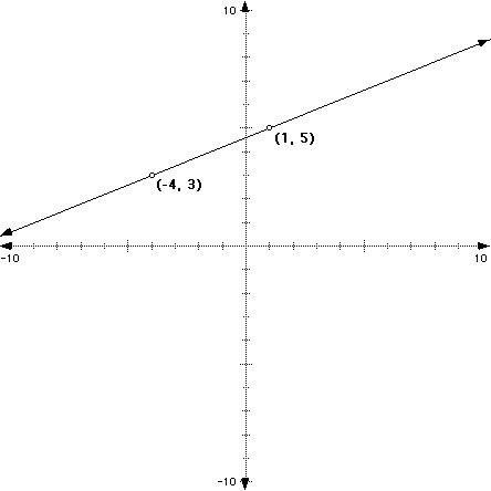
Notice right away that this is a positive slope.
Next, because the defintion of slope is "the change in y-values over the change is x-values" or,

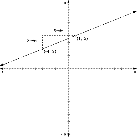
we can count up "rise vertcially" from the point (-4, 3) until we are abeam the point (1, 5) and then "run horizontally" over to the point (1, 5) to get our values for rise and run.
Look at the picture below. See, we "rise" 2 and then "run" 5 to get from one point to the next.
What about if we wanted to go from the point (1, 5) to (-4, 3) by moving left first then down? Well, it shouldn't make a difference how you move because the points are on the same line, but let's see:
If we started with the point (1, 5), we would move down vertically, which would give us a negative 2 movement. Then we would move right across to the point (-4, 3) which would give us a negative 5 movement as the illustration shows below.
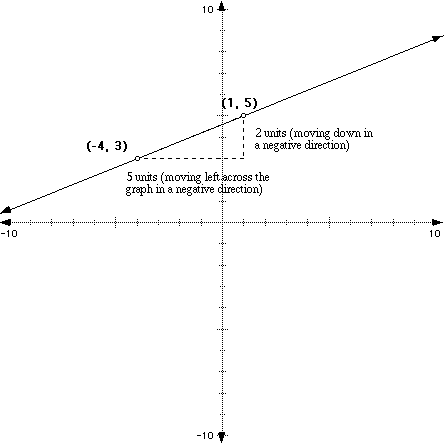
So if we move down 2 and then across negative 5, our change in y over the change in x would be -5/-2 which is 5/2. So, as long as you perform all of the movements and calculations correctly, it won't matter where you start and stop (which points you pick) on the graph when discovering the slope of the line between two points.
Now, algebraically, let's substitute the corresponding values of the coordinates into our slope formula:

So,

which is the same as we got graphically!
Also, find the slope between the points (5, 3) and (2, 2). If you plot these points, the first point (5, 3) is "up and diagonally to the right" of the second point (2, 2). However, after plotting these, it should be clear from the previous example that no matter what the order is of the points printed on paper, after graphing them, the rationale for positive and negative slopes must still "hold." Additionally, it should occur to you that in the general form of the slope equation, putting y1 or y2 first shouldn't matter, as long as you keep the same order for the denominator (x1 and x2). So, you can also write the slope equation as:

If you calculate the slope between the points (5, 3) and (2, 2) you should obtain a slope of 1/3 as illustrated below:

Examples for calculating the slope between two points:
Try calculating the slopes between the following points using the slope formula or graphically determining the slope as discussed above:
1. (1, 4) and (9, 2)
2. (5, 4) and (3, -2)
3. (-4, 7) and (1, -3)
Click here for the answers.
Zero slope
Plot the points (-1, 5) and (7, 5). After doing this, you should notice that if you construct a line between the two points, the line should be horizontal. Now, put your pencil on the point (-1, 5) and move it across the paper to the point (7, 5). Did you rise at all? You should have just moved horizontally along the paper from the point (-1, 5) to the point (7, 5). So, this means that you did not "rise" at all, but you "ran" 8 units across the graph. So, the slope would be 0/8 or 8 as shown below in the calculation.
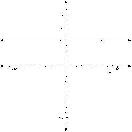

This will hold true for all horizontal lines. In other words, the slope of all horizontal lines is zero. This is a very important point in graphing functions! Note that when the y-values of two coordinates are the same for a linear function, they "subtract out" in the numerator of the slope, as any number minus itself is zero. So, for a short cut, you can remember that if any two points on a line have the same y value, the line will be horizontal.
Undefined Slope
Since the slope of a line is usually written as a fraction, like -2/5 or 3/1 to represent the rise over run concept, what would make a slope (a fraction) undefined? Clearly, it would be if zero appeared in the denominator as the only number. For example, the fractions 2/0, -1/0 and 0/0 are all undefined. Now, as a slope, the denominator represents the "run" of the slope as the definition of a slope is "rise" over "run" as stated previously. So, if we rise from one point to another on a line, but cannot run anywhere, we go straight up from one point to another and stay there. If you picture this, as illustrated below, it is a vertical line. Let's try an example. Graph the points (-2, 3) and (-2, 6) and then construct a line between the points. You should notice that going from one point to another you "rise" but do not "run" anywhere. Also, calculate the slope algebraically to make sure that you get "zero" in the denominator.
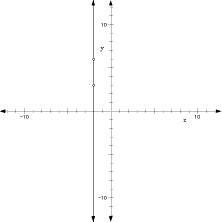

So, the slope of a vertical line is always undefined. Many people confuse zero slope with an undefined slope. Notice, however, that an undefined slope is the slope of a vertical line while a zero slope is the slope of a horizontal line which are TOTALLY different! Instead of memorizing: zero is to horizontal slope, as, undefined is to vertical slope, think of the definition of slope as the fraction or ratio rise over run and note when zero is in the denominator there is no run, just rising, so the result is a vertical line. On the other hand, if zero is in the numerator, there is no rise, just a run, so the result is a horizontal line. The concept is much easier to understand than it is to memorize! Also, note for a short cut, that if the x-values of two coordinates in a linear function are the same, when using the equation to calculate the slope, the x-values will subtract to equal zero, so the denominator will always be zero. So if the x-values are the same for the two coordinates when calculating the slope of a line, the line will be a vertical line.
We will see in the next lesson, "Algebraic Forms of Linear Functions," that when the equation of a line is solved for y, meaning that "y is by itself of the left- or right-hand-side of the equation," the coefficient of x is the slope of the line. For example, the slope of the line, y = -2x + 7 is m = -2, while the slope of the line y = (2/3)x - 1 is m = 2/3. If the equation is not solved for y, you must solve for y before determining the slope. For example, if the equation of the line was 3x + 2y = 7, we would solve for y, obtaining y = (-3/2)x + (7/2), so our slope would be m = -3/2.
Intercepts
Two very important areas of graphing lines are what are called the x- and y-intercepts. The definition of these terms is simply where the graph crosses the x- and y- axes, respectively.
The y-intercepts
If I tell you that the equation, y = -2x + 5 crosses the y-axis at (0, 5), you may not know anything else about the equation, but you will know that the equation crosses the y-axis at (0, 5). Notice that any point on the y-axis has the coordinate of the form (0, y). In other words, to plot a point on the y-axis, you do not move along the x-axis at all before going up or down to the point on the y-axis. Thus, the coordinate describing where the graph crosses the y-axis will always have a zero in the x-value of the coordinate. This also means that to find the y-intercept (where the graph crosses the y-axis) of any equation, you have to substitute zero in for x and then solve for y. So, for our example, if we substitute 0 in for x, we would get f(0) = -2(0) + 5 = 5. So, the actual y-intercept is (0, 5). A very important point to remember is that to find any y-intercept of any graph at any point in your mathematics career, you can substitute "0" in for x in any equation, solve for y, and that is the point where your graph crosses the y-axis. It may be a fact later in your mathematics career that there may be two or more y-intercepts, but you can find them all by substituting "0" in for x and solving for y.
Example: What is the y-intercept for the function y = 3x + 7?
To find the y-intercept, substitute zero in for x, solve for y and get: y = 3(0) + 7 = 7. So, the graph of the equation crosses the y-axis at the point (0, 7), and thus, has a y-intercept of (0, 7).
Example: What about 3x + 7y = 14?
To find the y-intercept, again, substitute 0 in for x and solve for y and get:
3(0) + 7y = 14,
so 7y = 14 (then divide each side by 7)
so y = 2.
Therefore, the graph of this equation crosses the y-axis at the point (0, 2), so the y-intercept of this equation is (0, 2).
The x-intercepts
If you can find the y-intercept, finding the x-intercept is just as simple. If I tell you that the same equation used above, y = -2x + 5, crosses the x-axis at the point (5/2, 0), and you know that it crosses the y-axis at (0, 5), you could draw the line containing those two points without ever having to find another point on the line! You could also find the slope of the line using the slope formula. If I said that the x-intercept was (5/2, 0), to find that, you would move from the origin to the right 5/2 or 2 and 1/2 units and not move up or down, as the point remains on the x-axis. All x-intercepts are in the form (x, 0), meaning that the y-value is always zero. So, to find the x-intercept of any equation, EVER, always substitute 0 in for y and solve for x. Note that if the equation is a function, y may be written as f(x). This is not a problem, just substitute 0 in for f(x).
An Example:
Find the x- and y-intercepts for the function, f(x) = (3/5)x + 5 and graph the equation using the intercepts. After you find the intercepts and graph the equation, click here to see if your answer is correct.
Exercises:
1. What is the x-intercept for the function y = 3x + 7?
2. What are both the x- and y-intercepts for the equation 3x - 2y = 4?
3. What is the x-intercept for the equation f(x) = 2x - 8?
4. What hare both the x- and y-intercepts for the equation f(x) = 2x?
The answers are, (-7/3, 0), (4/3, 0), (4, 0), and (0, 0), respectively. Note that because the last equation has a coordinate of (0, 0), the graph passes through the origin. Click here for detailed calculations for the x-intercepts (and some y-intercepts, too).
Practical uses of Graphing Functions
Graphing is used in real-life situations every day. For example, graphs of the stock market and NASDAQ are in the paper every day. Two important characteristics involving graphing are finding out where two lines meet and predicting future outcomes with graphs.
When Two Lines Meet
Graph the equations y = (4/3)x + 2 and y = -10x + 5 on the same line as indicated below.
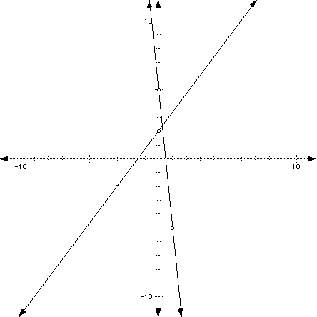
What are the x- and y-intercepts for the function y = (4/3)x + 2? What about the x- and y- intercepts for y = -10x + 5? What are the slopes for each of the functions?
If you look closely at the graph, it appears that the point where the two graphs meet is at about (1/3, 2 1/3). Sometimes it's hard to tell exactly where the lines meet by graphing, so in a later section, we'll show you how to find the intersection algebrically. This is important to understand. You must know how to find the solution (the values of x and y) of two equations. The solution of two equations is the value of x and y that satisfy both equations. For instance, if the solution of two equations was (2, 3), that means that when you substituted 2 into both equations for x, and solved for y, you would get 3.
Let's try an example here that will have a "friendly" result that we can see pretty well graphically.
Graph the equations of the lines y = 2x + 5 and y = (-3/2)x - 2. Notice that the slope of the first equation is 2 and the slope of the second equation is -3/2. Also, the y-intercept of the first equation is (0, 5) and is (0, -2) for the second equation. From this information, we can graph each line. Start by plotting the y-intercept for each equation separately and then from the y-intercept, say (0, 5) in the first equation, plot the next point by using the slope. So, start at the y-intercept (0, 5) and the from that y-intercept, rise 2 and run to the right 1 and plot your next point. You should be at the point (1, 7). Now, connect those points and you will have your first line!
For the second equation, y = (-3/2)x - 2, first plot the y-intercept (0, -2). Now, using the slope (-3/2), from the y-intercept, "rise NEGATIVELY" -3. So, you are moving down from the y-intercept. Then, run to the right 2 units and plot your point. You should be at the point (2, -5).
Check your graphs against the illustrations below.
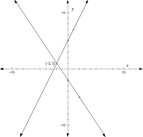
Notice that the lines meet at the point (-2, 1) as illustrated. In this graph, it's easy to tell where the lines meet. Sometimes, as seen previusly, it's not so easy to tell where the lines meet. That's why we'll show you another was (algebraically) how to find the point where they meet in a later section.
Predicting Future Outcomes.
Graphs of lines are very useful when predicting future outcomes. When a graph does not have a constant slope, for example, if it "zig-zags" like the graph of the stock market, predicting can be difficult. However, predicting outcomes using linear graphs is easy and quite useful.
For example, let's say, on average, that the average household income increases at a rate of $700 per year. If you start working at a rate of $20,000 per year, how much would you make a year in 15 years? In our example, the total salary is dependent on time, so time is the independent variable and salary is the dependent variable. (You may want to go back and review lesson 1 if you are struggling with the independent and dependent variables.) Our starting salary is $20,000, and increases at a rate of $700 per year, so we could make a function describing that relationship as f(t) = 700 t + 20,000. Now, if we wanted to predict how much we would make after the fifteenth year of work, we would simply substitute 15 in for "t" in our equation and obtain $30,500. Obviously this is a simplified example, as there may be several other factors affecting your income such as if your job pays on commission or offers bonuses. Let's graph this and see what we get. Since time is our independent variable, it is our standard "x" variable, so it is represented along the x- or horizontal axis. Since salary is dependent on time, it is our dependent variable represented along the y-axis.
Let's make a table of values in increments of 3 years:
| years |
|
|
|
|
|
f(0) = 700(0) + 20,000 |
|
|
|
|
f(3) = 700(3) + 20,000 |
|
|
|
|
f(6) = 700(6) + 20,000 |
|
|
|
|
f(9) = 700(9) + 20,000 |
|
|
|
|
f(12) = 700(12) + 20,000 |
|
|
|
|
f(15) = 700(15) + 20,000 |
|
|
|
|
f(21) = 700(18) + 20,000 |
|
|
Now, let's plot these points. Since we can't possibly make a y-axis that has several thousand units, we can plot the first two digits and say that the values are in hundreds of dollars, meaning that you will add three more digits when you are actually calculating the salary.
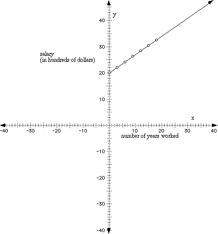
What is the domain of this function? Remember the domain includes all of the x-values or all of the independent variable values. So, it doesn't make sense to say that you are working "negative years," so the domain would run from 0 to whenever you quit or retired, say [0, 30]. Now, to calculate the range or the y-values, we know that at 0 years, the salary is $20,000 as shown. Now, for 30 years, we would just substitute 30 in for t in our original equation, f(t) = 700 t + 20,000 and get f(t) = 700(30) + 20,000 = 41,000. So after 30 years our salary would be $41,000, so the range of our function would be from [20,000 to 41,000].
A Practical Exercise:
Suppose you are about to graduate and are offered two jobs. Job A pays $32,000 and offers a raise of $850 per year. Job B starts off paying $27,500 with a raise of $1020 per year.
First, let's find the equations that represent each of the lines. The first equation would be represented by the equation y = 850x + 32000, while the second equation would be represented by y = 1020x + 27500.
How much would you be making at either job after 5 years?
At job A you would be making y = 850(5) + 32000 = $36,250, while at Job B you would be making y = 1020(5) + 27500 = $32,600.
So, after 5 years you would still be making less at Job B than Job A.
If you look at the two yearly raises, Job B offers more of a raise that Job A. Eventually, it should be obvious that Job B would "pass up" Job A with respect to salary. Let's graph the two lines to see if we can see how long it will take Job B (in blue) to pass Job A (in green) regarding salary.
We will plot the time (t) on the x-axis in years and salary on the y-axis in hundreds of dollars as in the example above. Let's make the domain approximately [0, 20].
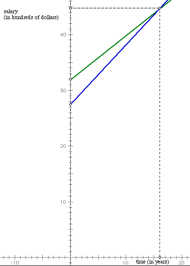
Notice that the lines meet (Job B starts to pass Job A) after about 16 years. We can tell this by plotting a point where the two lines intersect and drawing a vertical line down to the x-axis. To find the y-value (or what the salary is at the point where the graphs meet), draw a horizontal line over to the y-axis and read that value. In this case, the salary is a little less that $45, 000. So that means, that if you really liked Job B, you would have to work at Job for at least 16 years to make it worth your salary considering Job A. But, what about all of the years that you would have made more money working at Job A? Again, these are very simplified examples to allow you to see the foundation of graphing and the importance of being able to predict future outcomes. In the section "Linear Systems" we'll come back to this example to see how we can solve problems like this algebraically without graphing.
Something to think about... It would take you about 16 years working at Job B to match the salary of Job A. If you did work at Job B all of those years, how much money would you have lost considering that you made less at Job B for ALL of those years?