| Ia Hyperbola | 1b Box Maximization | II A New Look | III Past Discussions |
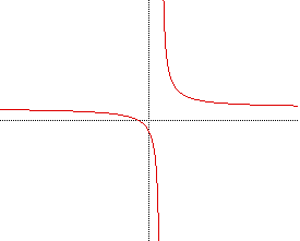
The graph of xy = c is a hyperbola, with the cordinate axes as the asymptotes.
The graph below is the graph of xy = 9. How can the graph be modified so
that the center of the hyperbola is not at the origin? If the equations
for a hyperbola centered at the point (h,k), that opens either vertically
or horizontally, are examined and expanded, they contain quadratic terms,
linear terms and a constant term.
In all the equations, h and k are constants that represent the coordinates
of the center of the hyperbola, a and b are also constants. 2a defines the
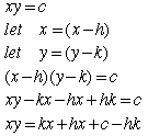
difference of the focal radii and b is defined in the equation ![]() where c is the distance from the center to the foci. The equation xy
= c, has a term of degree two, and a constant term, what it is missing is
linear terms. Equations in the form xy = ax + by + c will be examined to
determine the effect of adding linear terms. The first equation that we
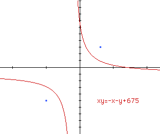
will examine is xy = x + y + 1.
where c is the distance from the center to the foci. The equation xy
= c, has a term of degree two, and a constant term, what it is missing is
linear terms. Equations in the form xy = ax + by + c will be examined to
determine the effect of adding linear terms. The first equation that we
will examine is xy = x + y + 1.
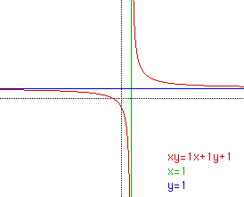
This graph is the graph of a hyperbola whose center has been shifted
from the origin. Let us briefly examine the math behin this shift. The equation
starts as xy = c, and the center is shifted by substituting (x-h) and (y-k)
for x and y.
From the last equation, the graphed hyperbola should be centered at (1,1).
In the terminology being used, k=a, h=b and the new constant ic c- hk. There
should be one vertical asymptote and one horizontal asymptote, with equations
y=1 and x=1. If the lines y=1 and x=1 are graphed, they appear to be the
asymptotes of the original graph.
The effects of changing a, b and c should now be examined. When the center
(h,k) is changed, the a and b change in the resulting equation. If a*b =
- c, the resulting equation can be factored and solved for the variables
x and y. The example below shows the factoring xy = -3x + 2y + 6.
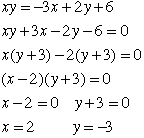
Whenthe equation xy = -3x+ 2y+6 is graphed, there should be a vertical
line, x = 2, and a vertical line, y =-3. As can be seen in the graph below,
this does occur. The preceding example is graphed in the color green. Several
other equations have been graphed demonstrating this behavior.
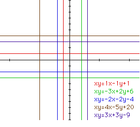
If a*b = - c, the result is two perpendicular lines intersecting at (b,a).
When a*b < - c and a*b > - c will also be examined. If a*b > -
c the graph will open towards the first and third quadrants, while if a*b
< - c, the graph graph will open towards the second and fourth quadrants.
The closer the product ab is to -c, the closer the foci of the hyperbolas
are to each other. As ab and c grow further apart, the hyperbolas' foci
spread out. This can be seen in the red, green and blue graphs, as well
as in the brown and purple graphs.
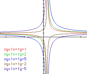
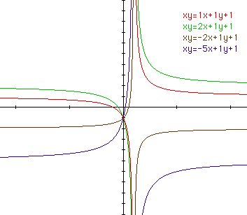
The majority of the equations graphed so far in this investigation have
had a=b. The relationship between a and b and the shape of the graph will
be examined. The coefficients a and b are give the coordinates of the center
of the hyperbola, (b,a). If either a or b is changed, the two transformations
of the graph occur. The first transformation that occurs is that either
the x or y coordinate of the center has changed. The other result is that
the product a*b has changed, so that the distance between the foci has changed
as well. This effect can be seen in the red and green hyperbolas, as well
as in the brown and blue hyperbols graphed below.
If the foci and difference between the foci are set, the hyperbola can
be graphed. An example is foci (-5,-5) and (3,3) and difference of focal
radii=8. The center should be at the point (-1,-1), the midpoint along the
segment between the foci. Using the definition of a hyperbola, the center
can be found.
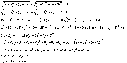
After completing the math above, the center is at (-1,-1). The graph
of the hyperbola is red, and the foci of the hyperbola are the blue points.
The previous mathematical derivation could be applied with variables
for the coordinates of the foci and difference of focal radii to determine
a general formula for a hyperbola whose foci are not on a horizontal or
vertical line.The same mathematical method could be applied to ellipses
to determine the general equation of an ellipse whose foci are not on a
horizontal or vertical line. The same method could also be used to find
the general formula for a parabola whose vertex, and focus are not on a
vertical or horizontal line.
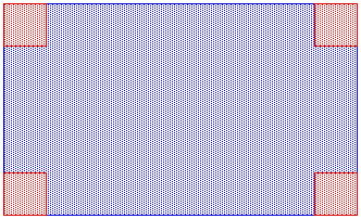
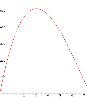
Most of the population would like to get the maximum return possible, with as little work or materials as necessary. An example problem that can be considered is the maximization of the volume of a box, given a flat sheet of cardboard to begin with. The box is created by removing the squares from each of the corners and folding up the sides. In the diagram below, the entire rectangle is the original sheet of material, the red squares at the corners are the material that would be removed and the white lines are where the folds would occur to create the sides.
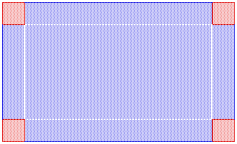
Geometer SketchPad was used to create the image above. GSP, if the construction
is done properly, will be able to animate the diagram to show the changing
of the size of the square. The diagram below shows the relative sizes of
the areas for the maximum volume of the box.
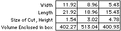
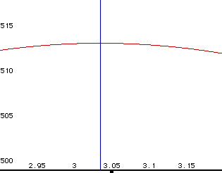
Another useful feature of GSP is that it will make tables of measured
values and calculations. One draw back is that it is extremely difficult
to get exact values this way. Unless the problem happens to have nice neat
solutions, the best GSP can do is approximate the answers. The table below
shows the values that I was able to measure using GSP, notice the inaccuracy
of the answers when a volume of 400 cubic inches was desired. 513.04 was
the largest volume that I was able to measure.
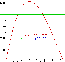
We need to look to methods that will overcome the weaknesses of GSP.
If an algebraic graphing program is used, by entering the correct equation,
we can get a graph that plots volume as a function of the size of a cut.
One nice feature of a graphical output is that it shows the pattern of the
change in the volume all at once. The graph can be interpreted using a straigth
edge to approximate the values of the volume and cut size.
One nice feature of a graphing program is that the range of the axis
can be manipulated allowing the region of interest to be focused upon. Another
feature is that lines can be graphed at exact values helping us with the
interpretation of the graph.
In the graph below, the green line would help us interpret when the volume
of the box is 400 cubic inches and the blue line would help us interpret
the maximum volume.
A third way that this problem can be examined is by using a spread sheet.
The spread sheet can be set up so that it will calculate the volume of a
box given original dimensions and the size of a cut. A nice feature of the
spread sheets is that the results can also be graphed to be interpreted
graphically.
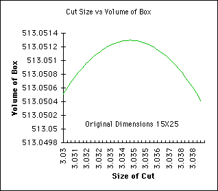
The spread sheet does not have to be graphed for the results to be identified.
In the cells that are used to calculate the volume, the highest value can
be identified. The size of the cut needed for any given volume will be displayed
numerically.
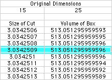
A nice feature of the spread sheet is that by varying the first cut and
by changing the size of the cuts, greater accuracy can be employed. In the
cells above, notice that the increment in the size of the cut is only increased
by 0.0000001 inches, and that the original cut size is fairly close to desired
value. This close examination can be done for any value of cut size. The
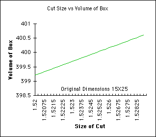
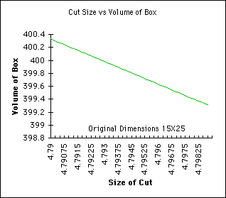
following graph shows the Volume of the Box as a function of the Cut Size.
Care needs to be exercised when the results are interpreted in any of
the three methods. By calculating the size of the cut to 7 decimal places
and the volume of the box to 12 decimal places in the spreadsheet, we may
be ignoring significant digits of the original dimensions. The uses of thw
information being calculated also needs to be considered. If an item is
being constructed using a yard stick and scissors, the accuracy is limited
to one decimal place, maybe two if we are lucky.
| Ia Hyperbola | 1b Box Maximization | II A New Look | III Past Discussions |
Return to Lars' student
page
Return to EMT 668 Page