 |
|
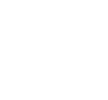
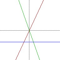
F(x) = 0x + 2 (Red) G(x) = 0x + 3 (Green) H(x) = ( 2)(3) = 6 (Blue) |
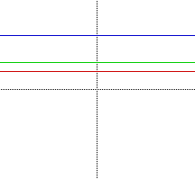
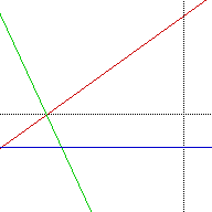
F(x) = 0x + 3 (Green) G(x) = 0x + 0 (Red under Blue) H(x) = (3)(0) = 0 (Blue) |
In section 1 we are asked to investigate the addition of two linear equations where H(x) = F(x) + G(x). This investigation led to no interesting discoveries. The sum of two linear equations is always a linear equation. Similarly section 4, we were asked to investigate the composite function between two linear equations where H(x) = F(G(x)). This investigation like section 1 produced little of note other than once again each new function H(x) was once again a linear function.
In this section we will divide the investigation into two parts, the case where H(x) = F(x)G(x) is not a quadratic, and the other where it is a quadratic. In both of these explorations we will be focus on the relationship between the two linear equations x & y intercepts and the newly formed quadratics x & y intercepts. The study will also look at using fewest amount of points to accomplish the common intercepts.
Terminology:
Linear Equation is any first degree polynomial. For ease of use and interpretation, I will write all linear equations in slope/intercept form. This form is written F(x) = mx + b where m is equal to the slope and b is equation to the y intercept value.
Product of two linear equations: Given that F(x) and G(x) are linear equations, their product is written in the form H(x) = F(x)G(x). H(x) is the newly formed equation that is the product of the two linear equations.
Intercepts: The intercepts of a graph are the locations on the x and y axis where the relation intersect with it. In case of a quadratic equation, its x intercepts if they are present are sometimes referred to as the roots of the equation.
Special Lines: Vertical and horizontal lines are sometime referred to as "special" lines. This is because their attributes and description are a little bit different from the sloped lines. A horizontal line has a slope of zero, and thus when written in slope intercept form looks like y = 0x + b or simplified y = b. A vertical line has an undefined slope of 90 degrees and is written in a similar form x = n, where n is a constant value.
Given two linear equations F(x)= mx + b and G(x) = cx + k, the product H(x) = (mx + b)(cx + k) creates a shape other than a quadratic when the slope for one or both of the lines is zero. The product produces a horizontal line, one of those "special" lines. Thus the product of two horizontal lines is again a horizontal line.
Now let use examine the two linear equations and their product in terms of intercepts.
| |
|
F(x) = 0x + 2 (Red) G(x) = 0x + 3 (Green) H(x) = ( 2)(3) = 6 (Blue) |
F(x) = 0x + 3 (Green) G(x) = 0x + 0 (Red under Blue) H(x) = (3)(0) = 0 (Blue) |
SUMMARY: One common y intercept is created when G(x) or F(x) is equal to zero. A second situation that gives a similar result as case (b) is when G(x) has a k value of +1. The product would always map itself onto the F(x) line, thus giving one common y intercept.
 | |
SUMMARY: Under the above mentioned conditions we can at most create a single point in common. In case (b) we had one y intercept and in case (c) we had one x intercept that was shared between the product and one of the linear equations. This exploration will not continue with vertical lines in that a very similar result occurs.
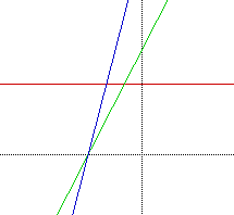
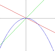
Given two linear equations F(x)= mx + b and G(x) = cx + k, the product H(x) = (mx + b)(cx + k) produces a quadratic when there exists a slope other than zero or 90 for both equations. Under these conditions (both have slopes other than 0 or 90), the product of two linear equations creates a quadratic equation. We will now explore the relationship of the intercepts between the product and the linear equations that make it up. We will track two things
Now let use examine the two linear equations and the product in terms of intercepts.
 |
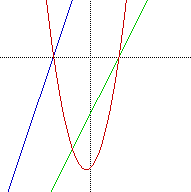 |
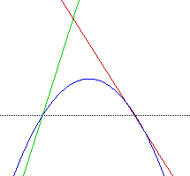
SUMMARY: The roots of the quadratic equation will always coincide with the x intercepts of the two linear equations. This happens because solving for the roots of the equation is the same process and determining the x intercepts for the linear equations
Thus for all cases from here on we will see that the roots of the quadratic will always intersect with the linear equations at the x intercepts. Thus both x intercepts will be in common.
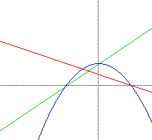 | |
SUMMARY: The case of two x intercepts and one y intercept in common is created every time that one of the linear equations has a value of one for the of its y intercept. The quadratic will share the y intercept with the linear equation that has a value not equal to 1.
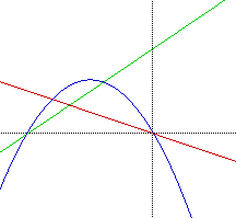 | |
SUMMARY: A linear equation of the form F(x) = mx + 0 eliminates the constant term from its product. (0,0) is a solution for F(x) and also for H(x), thus creating a common point.
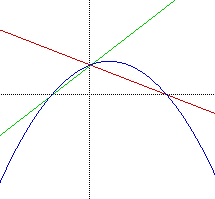 | |
SUMMARY: The intersection of the H(x)'s y intercept is equal to both of the linear equation's y intercepts when the two linear equations y = mx + b and y = cx + k have both k and b equal to 1.
 | |
SUMMARY: Setting the values of b and k to zero in the linear equations y = mx + b and y = cx + k, the product is a quadratic with no linear term and no constant term. This will always create a quadratic function that has a vertex of (0,0) that intersects with the other two lines at that point.
In this section we will divide the investigation into two parts, the case where H(x) = F(x)/G(x) is not a inverse function, and the other where it is a inverse. In both of these explorations we will be focus on how through manipulation of certain variables in the linear equations we can alter and transform H(x).
Terminology
Asymptote: is a line which a relation or function may approach but never touches. Asymptotes are often used in defining the domain and range of a relation. Algebra Xpresser draws a line connecting the two lines that approach the asymptote - this is not a correct thing to do and we will disregard that part of the diagram.
Inverse Function: is a function
which can be written of the form ![]() We will look at some of its characteristics
when manipulating the two lines that make it up.
We will look at some of its characteristics
when manipulating the two lines that make it up.
Given two linear equations F(x)= mx + b and G(x) = cx + k, the quotient H(x) = (mx + b)/(cx + k) creates a relationship that is not an inverse function when k and b are equal to zero or more generally, any time that the x variable can be canceled out of the equation.
 |
 |
Given two linear equations F(x)= mx + b and G(x) = cx + k, the quotient H(x) = (mx + b)/(cx + k) is an inverse function when k and b are not equal to zero or more generally, any time that the x variable can not be canceled out of the equation.
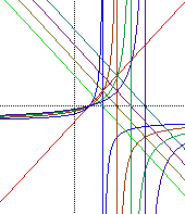
The graph to the left is a typical representation of the quotient of two linear equations where the x variable is not canceled out. All graphs of this type create the case where one of lines will intersect with the inverse function at the x intercept. This result occurs when
= 0, or in other words when mx + b = 0 (x intercept of the line)
Note: The blue line is not apart of the graph of the inverse function. If anything this line shows us an approximation of the vertical asymptote.
For the manipulation of the following linear equations and their impact on the inverse function I will commonly refer to the following equation and its variables.
I will begin each manipulation with the standard the below reference inverse function. That way we can notice the effects of the change more easily.
| Key pieces of information about the Baseline Inverse Function | |
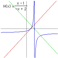 |
X Intercept when x - 1 = 0, thus x =1, (1,0)
Vertical Asymptote when -x + 2 =0, thus x = 2
Horizontal Asymptote when x approaches infinity is y = -1
|
Manipulation #1 - Altering the values of b in the equation
![]()
| (b) Manipulation of b, where b becomes more + | (c) Manipulation of b, where b becomes more - | |
| |
 |
 |
SUMMARY: Starting with the
equation![]() we manipulate the -1 in the numerator.
Before looking specifically at the diagrams provided was can note that by
manipulating the numerator we will be altering the x intercept of the inverse
function. It will still hold that the x intercept of the linear equation
will be shared with the x intercept of the inverse function.
we manipulate the -1 in the numerator.
Before looking specifically at the diagrams provided was can note that by
manipulating the numerator we will be altering the x intercept of the inverse
function. It will still hold that the x intercept of the linear equation
will be shared with the x intercept of the inverse function.
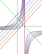
Diagram (b) is the case where we manipulate the numerator, x, x+1, x+2, x+3, .... The vertical asymptote is held constant and the pattern for the function seems to approach the horizontal asymptote at a different rate.
Diagram (c) is the case where we manipulate the numerator, x-2, x-3, x-4, x-5...... One interesting result of this manipulation is that a green horizontal line is formed when the numerator is x - 2. This result was actually discussed in Case 3.1 where the x variable can be canceled out of the function.
After finding this "special" line the function moved into the opposite two quadrants. This develops because the equation has a negative orientation.
Manipulation #2 - Altering the values of k in the equation
![]()
| (b) Manipulation of k, where k becomes more + | (c) Manipulation of k, where k becomes more - | |
| |
 |
 |
SUMMARY: Starting with the
equation![]() we manipulate the +2 in the denominator.
Before looking specifically at the diagrams provided was can note that by
manipulating the denominator we will be altering the vertical asymptote
of the inverse function. The x intercept will be common amongst all inverse
functions because the numerator has been held constant.
we manipulate the +2 in the denominator.
Before looking specifically at the diagrams provided was can note that by
manipulating the denominator we will be altering the vertical asymptote
of the inverse function. The x intercept will be common amongst all inverse
functions because the numerator has been held constant.
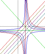
Diagram (b) is the case where we manipulate the denominator, -x+3, -x+4, -x+5, .... The vertical asymptote shifts to the right and the x intercept does not change.
Diagram (c) is the case where we manipulate the denominator, -x+1, -x, -x-1,- x-2, -x-3...... One interesting result of this manipulation is that a orange horizontal line is formed when the numerator is -x + 1. This result was actually discussed in Case 3.1 where the x variable can be canceled out of the function.
After finding this "special" line the function moved into the opposite two quadrants. This develops because the equation has a negative orientation.
For the sake of our investigation we will finish with the manipulation of only the constant terms. Manipulating the constant term we are able to show the progression from an inverse function (in two quadrants) to the linear equation that divides them, and then again to an inverse function (in the opposite two quadrants). The vertical line that divides the transition is when the x variable can be canceled out of the function.