I chose to explore the following equation from assignment 2.

in the case where b = 1 & c = 2 and a varies.

First, I selected a range of values for the variable a (-2, -1, 0, 1, & 2) and graphed each the equations separately. See the equations and their respective graphs below.

For a = -2,

For a = -1,

For a = 0,

For a = 1,

For a = 2,

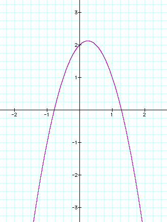
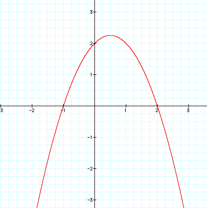
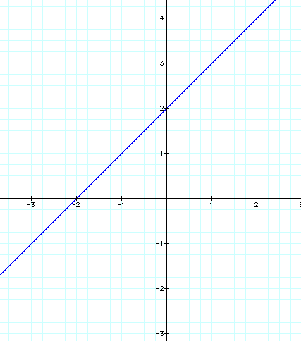
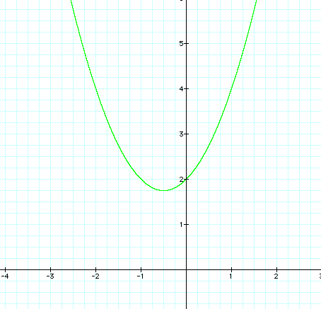
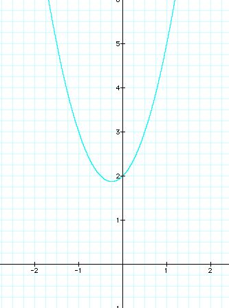
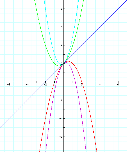
The common point to all 5 of these graphs is the coordinate point where x = 0 & y = 2 or designated as (0,2).

Notice that when a is positive (a=1, a=2), the function forms a parabola that is concave-up and when a is negative (a=-1, a=-2), this function forms a concave-down parabola. Also, note that when a = 0, the function becomes a linear equation as follows:

with a slope = 1 and y-intercept = 2.

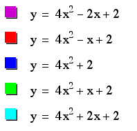
Let's explore this equation, , even further by holding the variables a & c constant while varying the b variable. If we set a=4 and c=2 and let O vary from -2 through +2, our new equations and the respective graphs would look like :

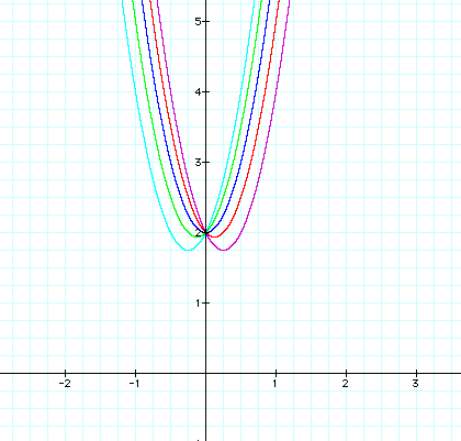
We can see from the graph that if we hold a & c constant and only vary b, the shape of the graphs remain the same. They are all parabolas. However, different values for b causes the function to move slightly up and down vertically as well as horizontally. For example, when b is negative, the vertex is to the right of the y-axis. When b is positive, the vertex is found to the left of the y-axis. Finally, when b is equal to 0, the vertex of the parabola lies on the y-axis at the point (0,2) . This would make sense, because if we look at our equation (where b=0) and find the value for y when x=0, then y=2.

then y=2, when x=0

Return to Keri's Home Page