Assignment 11 Problems addressed: Polar Equation of a straight line and Problem 1 Cristina Aurrecoechea Fall 2005

(Before addressing the specific Problems as stated in the Assignment, I would like to address the polar equation of a straight line, question raised by Prof. Wilson in class.)

Equation of a straight line

My solution is expressed as a function of slope (m) and ordinate value for x=0 (n). The reasoning behind the equation is: given a straight line, and given any point (x,y) in it, r is the distance from origin (0,0) to (x,y). In other words, r is the hypotenuse of the right triangle whose sides lie on (1) the x axis, (2) the vertical line through the point (x,y), and (3) r. See Figure 1.

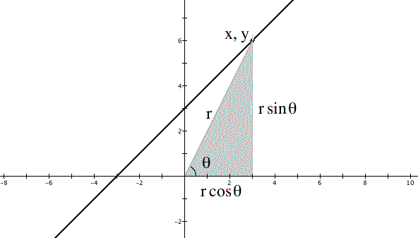
If we define theta q (attention: some browsers will display a q instead of the greek letter) the angle formed by the hypotenuse and the x axis, we know that:

and

Now we substitute x and y in the equation y = mx+n of a straight line --with m as slope and n as ordinate for x=0--, and we have the equation in polar coordinates.

There are some problems with this equation, though. It cannot describe

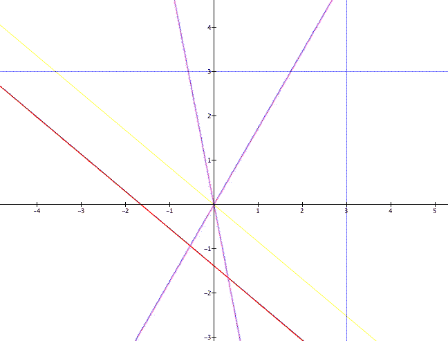
Please click in this gcf file to see the polar equations of different lines. Figure 2 is a graph obtained from this file. There are some interesting observations in how Graphic Calculator software behaves.

We show in red a line with slope m and ordinate (x=0) n. We provide a slider for m and n is the slider provided by Graphic Calculator that allows for animation. When n = 0, we do not see the line (as we said above, the equation does not provide for that case). So I added the green line (it might be yellow in your browser). Because it passes through (0,0) its equation is very simple: the angle q equal to a constant value, which depends on the slope m of the red line. Since m = tan(q), q = atan(m). Either expression can be used in Graphic Calculator to plot a straight line. But they do not behave equally. While the first one (that I used) gives you the whole line (for any value of r), the second one gives you a segment and allows you to increase the range of r values displayed.

Next I show in purple the equation of another line passing through (0,0), and make it rotate by using the n value just for the sake of animation. As you can check, these lines are really segments because of the type of equation I used.

Finally in blue I provide the equation for lines that are parallel to either axis using the equations provided above for x and y (after Figure 1).

Problem 1

We explore the polar equation:

We want to understand the effect of a,b, k and n in r. Also we want to understand the effect of using sin() instead of cos(). For this discussion we provide the following gcf file. We are plotting the values of r while the angle q vary from 0 to 2p.

Let's start with a = 0.

For k = 1 we have the equation of a circle tangent to an axis. See Figure 3.

• The effect of using cos() or sin() (shown in Figure 3) is to rotate the circle 90 degrees around the origin (0,0).
• The effect of b is simple: makes the r bigger or smaller, it is a module effect. In this case of a circle it is the diameter of the circle, the maximum value of the r.
• The effect of n is to rotate around the origin (pole).

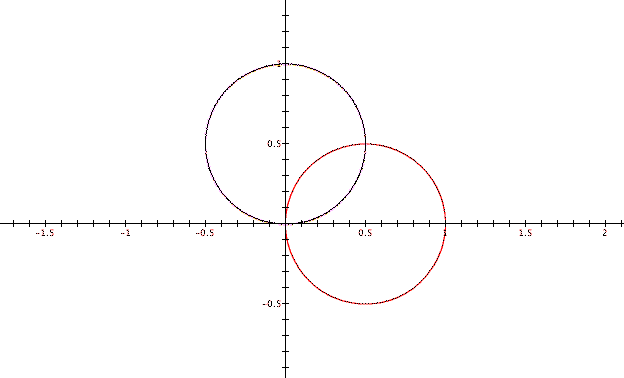
The most interesting effect is the one by k. Because it is multiplying the angle for which the cos() (or sin()) is calculated, its effect is like fitting several curves (deformed circles) in one rotation (one round around the origin, while the angle varies from 0 to 2p). It is the "leaf" effect. You could guess that if k = 2 you get two leaves, if k = 3 you get 3 leaves etc. Well, it works for k = odd numbers, but for k=even numbers the number of leaves is double! Why?

Looking at the effect of a helps in understanding what is happening. In reality the number of leaves is always twice k, but for k = odd numbers (1,3,5,...) you only see half of the leaves. The other half just happen to be located on top! For k = 1 in Figure 3 the circle is drawn twice: once while q varies from 0 to p, and again while varying from p to 2p. (You could check that if you keep the angle in between 0 and 3.14, for k = 2 you only see two leaves instead of four).

Now let's assume a is other than zero.

Let's start with k = 1.

As we increase a (a = 0.1) we see the two circles, one (smaller) inside the other. As a increases, this "leaf" gets smaller an smaller until it collapses into the pole (0,0) for a = 1.

For a > 1 the curve no longer crosses the pole. In fact, as a increases its value with respect to b, the curve ressembles a circle again. Why? Look at the equation: if a is >> than bcos(kq+n), the equation becomes simply r = a, which is the equation of a circle centered at the origin (0,0).

What is the effect of k when a is other than zero?

For a < 1 it is as before, the leaf effect: if q varies from 0 to 2p, the number of leaves is equal to 2k. Figure 4 shows:

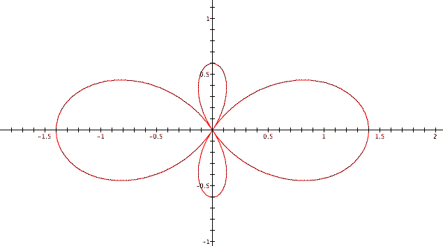
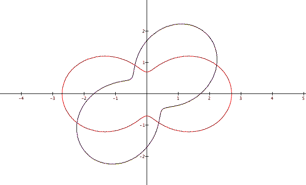
But for a > 1 the smaller leaves disappear and you see only two big leaves. For the specific case k = 2 the line adopts the shape of a peanut (see Figure 5).

Fun exercise.

Return to Cristina's page with all the assignments.