
OTP (Outside the
Parameter)
Presented by
Dana TeCroney
The
purpose of this investigation is to explore parametric equations using the
program Graphing Calculator.
Consider the equation ![]() . With many other graphing technologies such as the
TI calculators, this equation cannot be graphed (as is, parametric equations
are necessary), but can with Graphing Calculator.
. With many other graphing technologies such as the
TI calculators, this equation cannot be graphed (as is, parametric equations
are necessary), but can with Graphing Calculator.
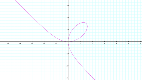
![]()
How
else could you deal with an equation like this?
If
we wrote this in parametric form would things change? Well, let's see shall we…
Let
y = tx, where t is our parameter.
Now, substituting for t, we obtain.
x3 + t3y3
= 3x2
With
a little algebra, it can be shown that:
 ,
, 
Now
things get interesting when we begin to graph this parametrically with
different ranges for t, start with t = 0 .. 1. In the following graphs, the pink is the original graph of ![]() and the blue graphs are the
parametric equations.
and the blue graphs are the
parametric equations.
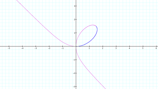
Obviously
this range isn't good enough, so try t = 0 … 10
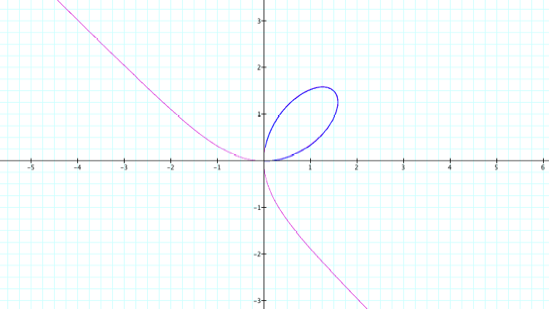
t
= 0 … 100?
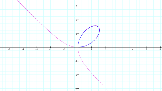
If
you look closely, this is actually a worse approximation of the original graph,
to illustrate the point, try t = 0 … 200.
You can see how the approximation is becoming more rigid and less
smooth.
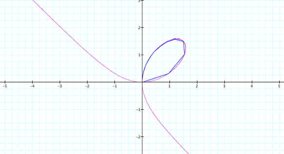
When
t = 0 … 1000, the approximation isn’t even close as shown below.
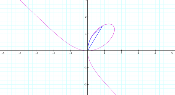
As
shown in the graphs above the best upper bound we have tried is t = 10, however
we have only covered the loop of the original graph. To cover the rest, we need to consider negative values of t,
however, there is a problem: domains.
In the original equation ![]() , the domain consists of all real numbers, however,
, the domain consists of all real numbers, however, ![]() ,
, ![]() , has a domain restriction of t not equaling -1. So, can we approximate the entire graph
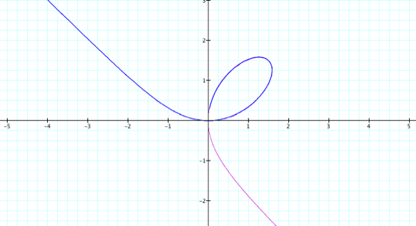
with a t value less than -1? The graph
below shows t = -.999 … 10.
, has a domain restriction of t not equaling -1. So, can we approximate the entire graph
with a t value less than -1? The graph
below shows t = -.999 … 10.
As
it turns out, t = -10 … 10 gives us an approximation for the whole graph, but
there is an extra line where the slant asymptote is…
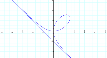
This
illustrates one of the limitations of technology. When graphing technologies are given parametric equations,
they evaluate a given number of points and then connect these points. So why the line? Consider the following.
 =
= ![]()
 =
= ![]()
As
you can see, as t gets really close to -1, the points are far off in the second
and forth quadrant depending on whether you are approaching from the left or
the right. When you put this all
together, the technology connects these points and hence the line, despite the
fact that the line (asymptote) isn’t part of the graph.