Assignment 1

The beauty of Calculus

This assignment analyses the non-linear curve

,

where a, b, and k are constants.

In particular, for (i.e., when ), the curve is symmetrical about the origin. When , or . Similarly when , or .

Further, when , the curve simplifies to . Since a and b are not equal in general, if and only if . In other words, the line is an asymptote to the curve, except at .

Let us observe the behavior of the curve as the values of a and b change.

CASE 1(a) , and , i.e.,

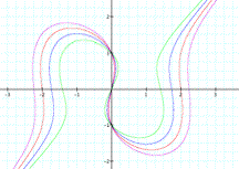
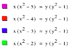
Figure 1.1

We observe that as the value of a increases, the curve expands along the x-axis.

CASE 1(b) , and , i.e.,

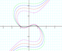
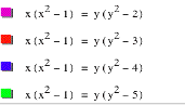
Figure 1.2

We observe that as the value of b increases, the curve expands along the y-axis.

CASE 2 , i.e.,

or

Factorizing the left hand side gives, .

Thus, provided . The ellipse corresponding to and the asymptote for different values of a and b are shown in Figure 1.3.

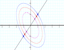
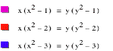
Figure 1.3

To have a better understanding of the behavior of the curve when , let us consider an example, say and in CASE 2a below

CASE 2a , and

We fix the value of b at 1 and observe what happens as ‘a’ tends to 1 from the left hand side and right hand side (Figure 1.4). We see that as ‘a’ approaches 1 from either side, the original curve tends to an ellipse.

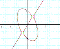
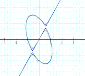
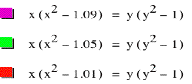
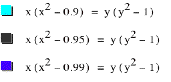
Figure 1.4

Click HERE for animation

Now let us observe what happens when ‘a’ is negative and ‘b’ is fixed at 1 in CASE 3 below.

CASE 3 , and , i.e.,

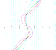
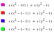
Figure 1.5

Figure 1.5 shows that as the value of ‘a’ decreases from 0 to -3, the curve regresses towards the y-axis.

Another interesting set of observations can be made when we consider the curve as illustrated in CASE 4 below.

CASE 4 , , and i.e.,

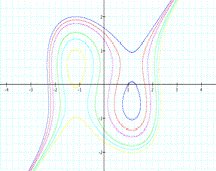
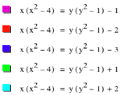
Figure 1.6

Observe the symmetry in Figure 1.6 when and or when and i.e., for corresponding positive and negative values of k. The generation of the loop for particular values of k is discussed below.

CASE 5 The behavior of when

The ‘sorter values’ in graphic calculator show that the curve splits at one point in the range as shown in Figure 1.7 below

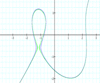
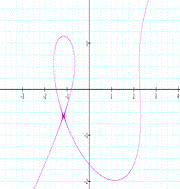
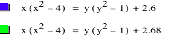
Figure 1.7

Click HERE for animation

To have the precise breaking point (as per the accuracy of the graphic calculator), we have plotted the following curves, and in Figure 1.8.

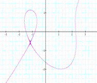
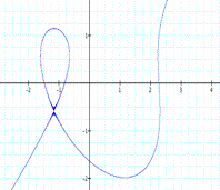
Figure 1.8

We observe that the curve splits at the point where . We have also investigated the case when k is negative and the curve splits at .

Why does the curve split?

The equation can be written as . To understand the behavior of the curve, let us fix the values of x and k, i.e., consider the equation or , where the constant .

The cubic equation may have one real root or three real roots (where two of them may be equal).

Consider the curves

(1)

(2)

(3)

A plot of equations (1), (2), and (3) is shown in Figure 1.8a.

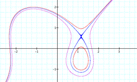
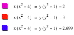
Figure 1.8a

Using with , equations (1), (2) and (3) can be written as

or (4)

or (5)

or (6)

A plot of equations (4), (5), and (6) is shown in Figure 1.8b.

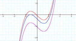
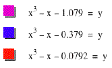
Figure 1.8b

Comparing Figure 1.8a and Figure 1.8b, we observe that the curve splits when has repeated roots. In the foregoing example, this occurs when . When has three real distinct roots, we have a loop.

Click HERE for a three dimensional view of the curve.

This assignment has revealed some of the insightful features of the curve . However, the exploration can be extended.

References

Finney, R.L., Weir, M.D., Giordano, F.R. (2001) Thomas’ Calculus, 10^th ed. Boston: Addison Wesley

Kline, M. (1977) Calculus: An intuitive and physical approach, 2^nd ed. New York: John Wiley and Sons

30 September 2006

Ajay Ramful

RETURN