![]()
Eric Gold
Assignment 2, Question
1:
Graphing Parabolas
1. Examine graphs for the parabola for different values
of a, b, and c. (a, b, c can be any rational numbers).
Try using the GC animation by replacing a, b, or c with an n and
selecting an appropriate range for n.
In studying parabolas and their
graphs, or the graphs of any function or relation for that matter, it is useful
to understand the implications of changing coefficients on both the function
and its graph. It is probably safe to say that most Algebra I students, and
likely many students in courses that were once called PreAlgebra, would
recognize an equation of the form
y = mx + b
and it is
likely that they would either remember or be able to deduce that m is the
slope, or rate of change of the function, and b is the y- intercept. Hopefully
they would also remember that the x-intercept is easy to find by setting y = 0
and solving for x. Unfortunately, this becomes more challenging for these
students when confronted with a linear equation presented in either in standard
form, Ax + By + C = 0, or as a point-slope equation, y - y1 = m (x
– x1). It is too
often the case that students either can’t see the relations that exist or they
have no interest in such concepts and investigations. If they were encouraged
along these lines, particularly if they were encouraged with an emphasis on
understanding what they are working with and seeing, it may heighten their
interest in the material and help them see that there are, in fact, reasons for
studying the material.
Considering that students are
poorly informed regarding linear equations, one can assume that they are
baffled and befuddled when looking at an equation of the form
Ax2
+ Bx + C = y.
Based on personal experience,
they seem to pretty much want to run out of the room screaming when confronted
with something on the order of
y = (x - h)2 + k.
Given the equation
![]()
they are
overwhelmed by the symbolism, let alone what the equation means. They don’t
have much of a concept of what happened to the y or what the equation is even
telling them.
If we as educators better
understand parabolas, i.e. the graphs of quadratic equations, perhaps we can help our
students better understand the materials and subject matter they are working
with.
Now we can consider the general
quadratic equation,
Ax2
+ Bx + C = y.
In
particular, we can consider the graph of the equation and observe how the graph
changes as we vary A, B, and C.
Then we can vary more than 1 parameter to see if what we’ve learned from
this experience holds if we apply it to more than one simultaneously varying
parameter.
A, the leading coefficient
What
are the consequences of varying A? As we can see from the graph below, changing
A changes the shape of the graph.
In particular, we have the following equations and graph:


If we look at the
original equation, i.e., the standard form of the quadratic equation, the influence of
A on the graph becomes more apparent. In particular,
when A > 0, the graph opens up. When A < 0, the graph opens down. When A
= 0, the quadratic term disappears and the equation becomes linear of
the form y = Bx + C, which is analogous to y = mx + b. A is the coefficient of the square, or leading,
term. One way of thinking about the leading term is that it leads, or drives,
the equation. If we were to construct a table of values of the function and
look at the quadratic and linear terms individually, it would be clear that as
x gets increasingly positive or negative, the quadratic term’s value grows
significantly faster than that of the linear term. When we compound this growth
by a factor of A, it further drives the value of the function and,
consequently, the shape of the graph. At the secondary level, this makes A
analogous to slope for a linear equation. If we take this to the next level and
consider this with more knowledge than a high school algebra student, we could
perform some simple analysis on the equation. For instance, remembering that
the first derivative tells us the slope of the tangent to the graph at any
given point. From the standard form of the quadratic equation, we find that the
derivative, y’, is 2Ax + B. The linear and constant terms have disappeared, and
the slope depends on x and its coefficient.
Notice what happens as we vary the leading coefficient in the following movie:
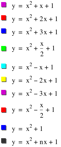
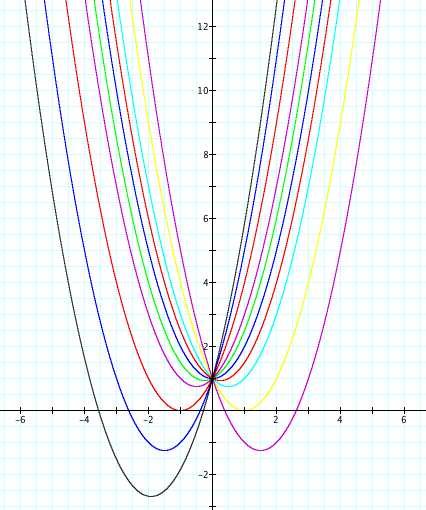
Notice: there are no apparent changes in the "size" or shape of the graph as there are when we changed A. In fact, it appears that the graphs are just shifting left and/or right. Notice also that all the functions go through the point (0,1). Why do both of these happen?
Let us first consider that all graphs go through the point (0,1). Note that for any of the individual curves in this family of functions has a constant term 1. Thus, if we let x = 0, each of these functions has a y-intercept of 1. In fact, this can be clearly seen in the animation below, where the black line represents the graph of the function ![]() .
.
When we compare what happens when we vary B, why is it so different than when we change A? Perhaps we should consider what we learned in Algebra 1 about transformations of functions. We know that in order to have a horizontal shift, we need to operate on x, say consider the function f(x-h). This will produce a horizontal shift of h units. The question now becomes what is the impact of changing B on the horizontal shift of the function? Let us consider the equations ![]() and
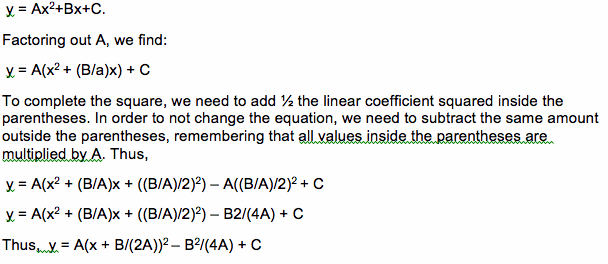
and![]() . They can be found on the graph above, the former in blue and the latter in red. You would expect, if B represents the horizontal shift, to be 2 units (from 0 to 2), but this is clearly not the case. In fact, when we consider the graph, the horizontal shift has been 1 unit to the left. Why is this so? Perhaps we should reconsider the original equation: Ax2 + Bx + C = y. In order to more clearly see what's going on, let us use some algrebra to manipulate the equation into a form that makes sense. In particular, since we want to find an equation of the form y = f(x-h), let's complete the square and see what we can...
. They can be found on the graph above, the former in blue and the latter in red. You would expect, if B represents the horizontal shift, to be 2 units (from 0 to 2), but this is clearly not the case. In fact, when we consider the graph, the horizontal shift has been 1 unit to the left. Why is this so? Perhaps we should reconsider the original equation: Ax2 + Bx + C = y. In order to more clearly see what's going on, let us use some algrebra to manipulate the equation into a form that makes sense. In particular, since we want to find an equation of the form y = f(x-h), let's complete the square and see what we can...
.
C, The Constant
Finally, we consider C, the constant. What are the implications of varying C? Consider the following diagram and variations on the equation x2 + 2x + C = y
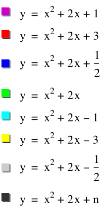
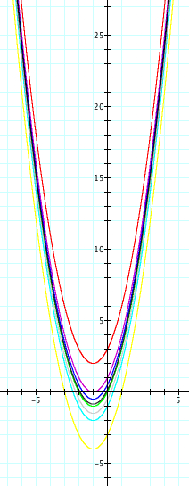
Note the only change as we go from graph to graph is a vertical shift. Quite simply, this is because the linear and quadratic terms establish the shape and horizontal position of the graph and are driven by x. However, when we let x go to 0, the constant term is all we have to drive y. Thus, whatever C, our constant term, is will determine the vertical position of the graph of the function. Observe:
Putting it all together
Above we looked at each of the "constant" terms in a quadratic equation, A, B, and C, and discussed their impact on the graph of the function. Now, we can put everything together. Observe the graph and related equations:
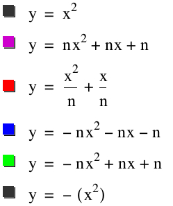
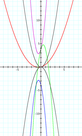
It is not unreasonable to expect that varying A, B, and C simultaneously will cause the graph of the function to change consistent with the various actions happening concurrently, as demonstrated below:
