
Polar Equations
By Pei-Chun Shih
The polar
coordinate system is a
two-dimensional coordinate system in which the position of an object is
recorded using the distance from a
fixed point and an angle made with a
fixed ray from that point. Since distances and angles are the main components
of the polar coordinate system, this system is especially useful under the
circumstances where the relationship between two points is most easily
expressed in terms of angles and distances.

In
the polar coordinate system above, a fixed point O is called the pole (origin). A horizontal ray directed from the pole
toward the right is called the polar axis. If a point P has polar
coordinates (r, ![]() ), then the
distance from the pole to point P is | r | and the angle formed by OP and the
polar axis is
), then the
distance from the pole to point P is | r | and the angle formed by OP and the
polar axis is ![]() . Note that the
angle,
. Note that the
angle, ![]() , can be
measured in degrees or radians.
, can be
measured in degrees or radians.
An
equation expressed in terms of polar coordinates is called a polar equation. As mentioned earlier, distances and angles are two
main elements of the polar coordinate system and therefore a polar equation can
be specified by defining r (distances) as a function of ![]() (angles) in many cases. For example, r =
3 cos (
(angles) in many cases. For example, r =
3 cos (![]() ) is a polar
equation. A plot of all points whose coordinates (r,
) is a polar
equation. A plot of all points whose coordinates (r, ![]() ) satisfy a
given polar equation is called a polar graph.
) satisfy a
given polar equation is called a polar graph.
I am
going to explore some polar equations and their polar graphs in the following
sections.
Let’s
start with the simplest polar equation r = b
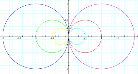
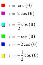
cos (![]() ). The graph is shown below. Notice that this graph are
circles with diameters of b unit
and pass through the origin. Also, the positive and negative signs of b determine the locations of the circles. When b is positive, the circles are on the right of the
y-axis and the circles are on the left of the y-axis when b is negative.
). The graph is shown below. Notice that this graph are
circles with diameters of b unit
and pass through the origin. Also, the positive and negative signs of b determine the locations of the circles. When b is positive, the circles are on the right of the
y-axis and the circles are on the left of the y-axis when b is negative.
[r = b cos (![]() )]
)]
Now
we know that we can alter the position and the size of a polar graph by
multiplying the function by a number. Next, we are going to explore the polar
graph of r = b cos (![]() ) by adding the
function by a number, say a. The polar graph of
) by adding the
function by a number, say a. The polar graph of
r
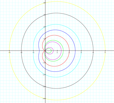
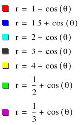
= a + b cos (![]() ) below are curves with different shapes. When a is smaller than 1, the polar equation r = a + b cos (
) below are curves with different shapes. When a is smaller than 1, the polar equation r = a + b cos (![]() ) forms curves
that have inner loops like the green and the pink ones below. When 1
) forms curves
that have inner loops like the green and the pink ones below. When 1 ![]() a
a ![]() 2, it forms curves that have dimples
like the red, the dark blue, and the light blue ones. When a
is larger than 2, the curves just curve outward without inner loops or dimples.
All the curves form by the polar equation r = a + cos (
2, it forms curves that have dimples
like the red, the dark blue, and the light blue ones. When a
is larger than 2, the curves just curve outward without inner loops or dimples.
All the curves form by the polar equation r = a + cos (![]() ) are called limacon (pronounced lee muh SOHN).
) are called limacon (pronounced lee muh SOHN).
[r = a + b cos(![]() )]
)]
How
about multiply ![]() by a number k
to alter the graphs of the two polar equations above? Let’s exam the polar
equation r = b cos (k
by a number k
to alter the graphs of the two polar equations above? Let’s exam the polar
equation r = b cos (k![]() ) first. Since b only determines the location and the size of r = b
cos (k
) first. Since b only determines the location and the size of r = b
cos (k![]() ), let b = 1 to simplify our exploration.
), let b = 1 to simplify our exploration.
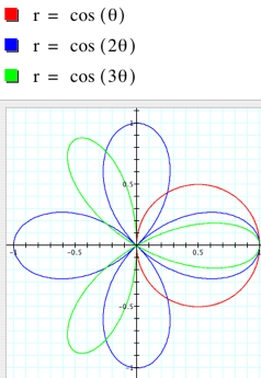
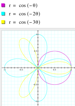
[r = cos (k![]() )]
)]
From
the two graphs above, we can see that multiply ![]() by k form petal shape curves. This type of curve is called
a rose. It seems like
whether k is positive or
negative, it has nothing to do with the shape of the rose curves. Therefore, we
will use only positive k in
the rest of our exploration.
by k form petal shape curves. This type of curve is called
a rose. It seems like
whether k is positive or
negative, it has nothing to do with the shape of the rose curves. Therefore, we
will use only positive k in
the rest of our exploration.
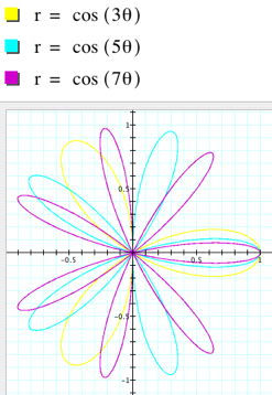
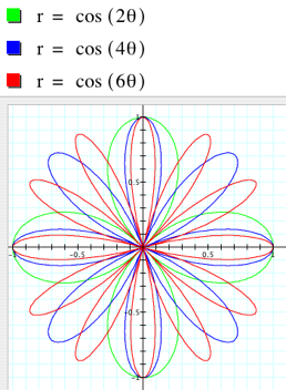
There
is an interesting finding here, the number of petals of a rose is determined by
whether k is an odd number
or an even number. When k
is an odd number, there are k
petals in a rose curve. When k
is an even number, there are 2k petals in a rose. Please look at the graphs below for the differences.
[r = cos (k![]() )]
)]
Now,
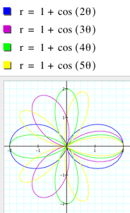
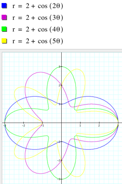
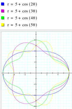
it’s time to explore r = a + b cos (k![]() ). First, let a
= 1, 2, and 5 with b = 1 (again, b only affects the size of the curves), and
explore the curves when k = 2, 3, 4, and 5.
). First, let a
= 1, 2, and 5 with b = 1 (again, b only affects the size of the curves), and
explore the curves when k = 2, 3, 4, and 5.
[r = a + cos (k![]() ) where a = 1, 2, and 5]
) where a = 1, 2, and 5]
Recall
the shape of r = a + b cos (![]() ) is a limacon.
From the two graphs above, we can see that if
) is a limacon.
From the two graphs above, we can see that if ![]() is multiplied by k then the shape of y = a + b cos (
is multiplied by k then the shape of y = a + b cos (![]() ) changes
completely. It changes from a limacon to a “flower-petal” shape. Here k determines the number of “petal”. In the polar
equation r = a + b cos (k
) changes
completely. It changes from a limacon to a “flower-petal” shape. Here k determines the number of “petal”. In the polar
equation r = a + b cos (k![]() ), there are
exactly k “petals”.
Besides, when a = 1, the petals “tie” at the origin. When a is larger than 1, the “ties” disappear. Also, the
larger the value of a, the
smoother the curve becomes.
), there are
exactly k “petals”.
Besides, when a = 1, the petals “tie” at the origin. When a is larger than 1, the “ties” disappear. Also, the
larger the value of a, the
smoother the curve becomes.