
Assignment 1: Problem 2
Jason P. Pickhardt
Problem:
Make up linear functions f(x) and g(x). Explore, with different pairs of f(x) and g(x) the graphs for
i. h(x) = f(x) + g(x)
ii. h(x) = f(x).g(x)
iii. h(x) = f(x)/g(x)
iv. h(x) = f(g(x))
Summarize and illustrate.
Exploration:
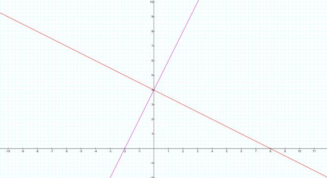
The following exploration was done in response to this problem. The first graph in a series illustrates the lines f(x) and g(x). The four graphs that follow are the graphs of the equations in the problem respectively. Also, the original linear equations are overlaid on each graph for the ease of comparison. At first, to conduct this exploration I simply created equations randomly out of thin air. After pondering what types of equations may give us an interesting result I was able to conclude that we can have three interesting relationships amongst the linear equations:
(1) Lines sharing one point of incidence.
(2) Parallel lines
(3) Perpendicular line
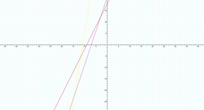
Case 1:
![]()
![]()
![]()
![]()
![]()
![]()
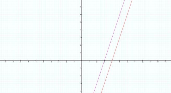
Case 2:
![]()
![]()
![]()
![]()
![]()
![]()
Case 3:
![]()
![]()
![]()
![]()
![]()
![]()
It seems that a good way to summarize findings for this exploration is to discuss each combination of the linear equations individually citing findings from all of the cases. Thus we will start in order.
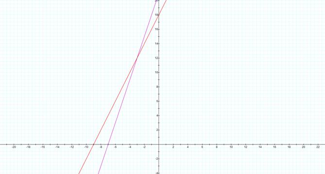
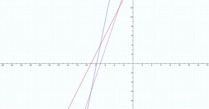
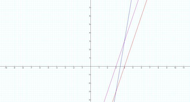
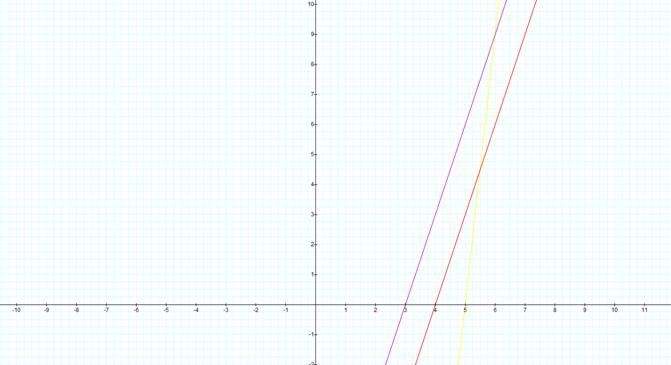
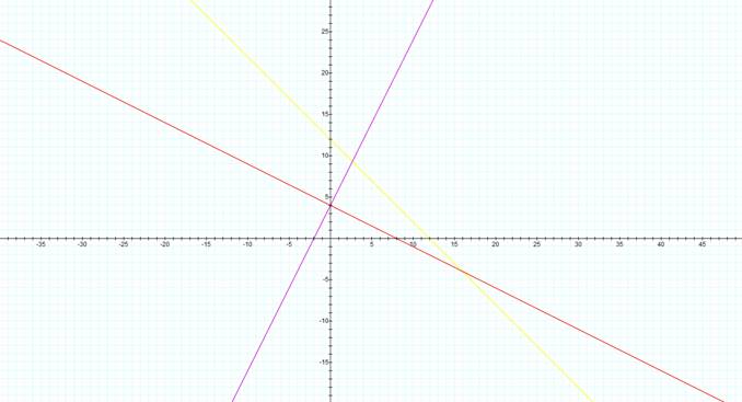
i) In the case where we are adding the two linear equations together, we do not really get a very interesting result. One notable observation that can be made across all three cases is that the new line seems to have one and only one point of incidence with the original two lines. This is the same whether the first two lines were parallel, perpendicular or already having a point of incidence. Also, it seems fairly obvious to note that the addition of two linear equations gives us a new linear equation. This is confirmed through both the equation for h(x) and the corresponding graph.
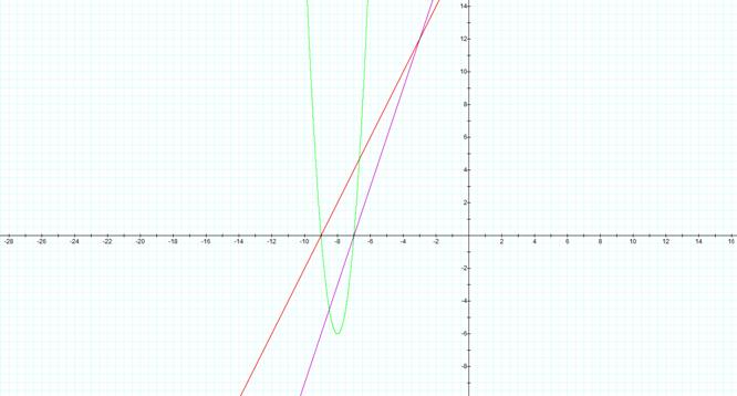
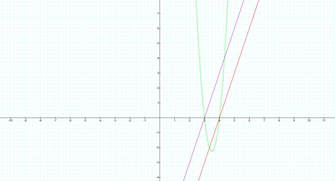
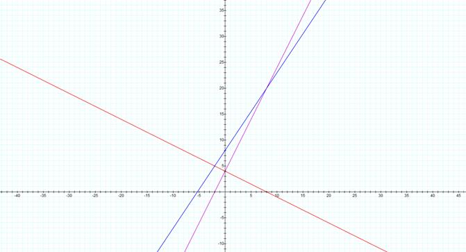
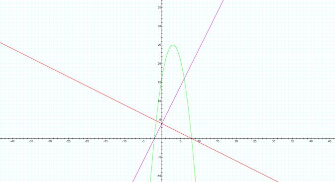
ii) This case is immediately far more interesting than the previous one. The multiplicative combination of the pairs of linear equations in each case yields a quadratic equation and subsequently a parabolic graph. The most interesting observation that can be made here is that the x intercepts of each of the linear equations are common to a root of the resulting quadratic equation. Let’s look at an example from case 1:

Solving the original equations for f(x) and g(x) to get x intercepts we get:


Now, to check that my assertion is true I can solve the new quadratic equation for its roots:
Here we see that the roots of the resulting quadratic are indeed the same as the two x intercepts of the original equations!
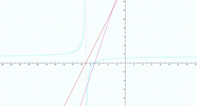
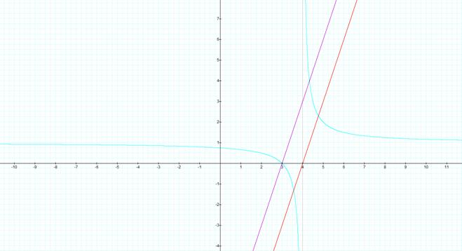
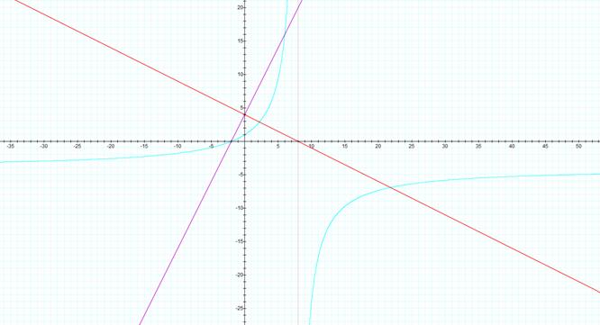
iii) In the case where we divide g(x) by f(x) we get another very interesting result. The resulting equation gives us a hyperbola. Also, similar to the previous combination there seems to be something going on with the original equations x intercepts. In this case the x intercept of one of the equations represents the value of the vertical asymptote of the new hyperbolic equation. Also, the remaining x intercept corresponds to an x intercept of the new equation. Here is an example from case 2:
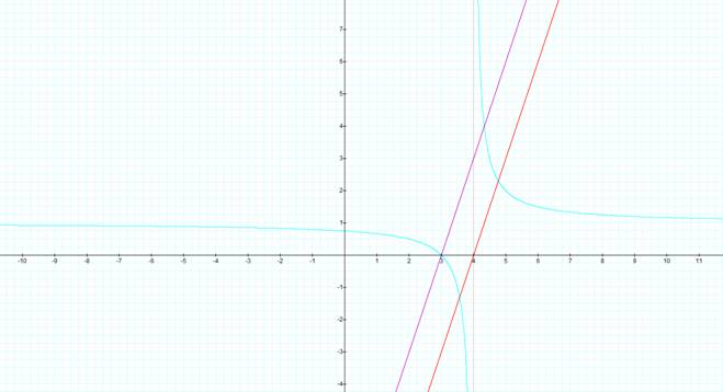
We can see that the red equations’ x intercept is the value of the vertical asymptote and the x intercept of the new equation is the same as the purple lines’. We can check this algebraically and also make a comment on why this is true. Finding the x intercepts of the original equations we get:


Now before trying to solve for the x intercept of the hyperbolic equation and its’ vertical asymptote let’s look logically at the equation:
![]()
We cannot have a 0 in the denominator of the equation and thus we cannot have the case where x=4. Thus we have confirmed that one of our intercepts is the value of the asymptote. However, this should be obvious given that g(x) was purposely put into the denominator and its’ x intercept is the value at which the equation is 0. Nevertheless it is important sometimes to discover things like this through hands on activity rather than by theoretical calculations. The same follows for the x intercept of the hyperbolic equation. When we set h(x) equal to 0 the denominator is lost through cross multiplication and we are simply looking for the zero of the equation in the numerator, which in our case is 3.
iv) At first glance plugging g(x) into the function f(x) for x seems like it would yield a very interesting result. However, this does not end up being the case. Similar to part (i), this combination yields a new linear equation. Also similar to part (i) this new line shares one and only one point in common with each of the two original equations.
Conclusion:
It is important to note that this could have been done without any graphing. We could have taken the general form of two equations f(x) =mx+b and g(x) =nx+d and manipulated them using the prescribed combinations. However, this is an alternate route that takes advantage of graphing technologies. With that said we can draw a few conclusions that are valuable from this exploration:
1) Adding, subtracting or taking f(x) and a function of g(x) will all yield a new linear equation with one and only one point in common with each original equation.
2) Multiplying two linear equations will yield a quadratic equation with roots equal to the two intercepts of the original equations.
3) Dividing two linear equations will yield a hyperbolic equation with x intercept equal to that of the numerator and value of the vertical asymptote equal to the x intercept of the denominator.
a. This can yield a trivial case in which the resulting division gives us a whole number or fraction of a whole number. In this case we will be graphing a horizontal line at the y value of this number.