
Assignment 10

By: Erica Fletcher
In this assignment we will investigate parametric equations. A parametric curve in the plane is a pair of functions
x = f(t)
y = g(t)
where the two continuous functions define ordered pairs (x, y). The two equations are typically called the parametric equations of a curve. The variable t is called a parameter and the relations between x, y and t are called parametric equations.In many applications, we think of x and y "varying with the time t." Thus we can make the ordered pair (x, y) vary with t.
Various graphing technology can be promptly used with parametric equations but we will use Graphing Calculator 4.0.
For various a and b, we will investigate
x = a cos(t)
y = b sin (t)
for![]()
for different values of a and b. What is the curve when a = b? a < b? a > b?

Let's first explore the graph of the parametric equation given by
x = cos (t)
y = sin (t)
for ![]() .
.
Here we will look at the following parametric equation:
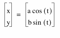
First we will look at what happens when a = b. In this specific case we will look at a = b = 1. The resulting graph is below.
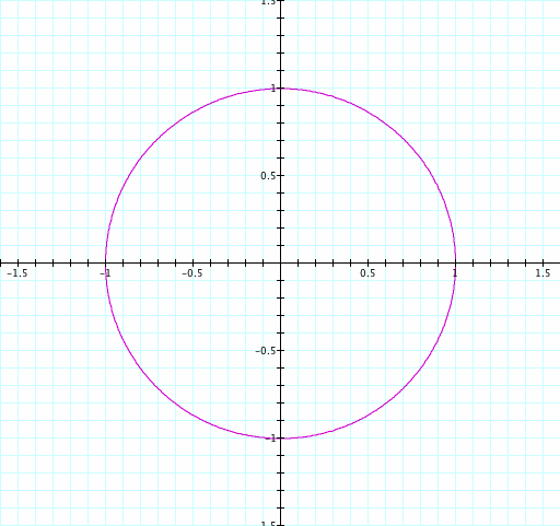
We observe that it makes the graph of a circle with a radius of 1. Given a parametric curve, sometimes we can eliminate t and obtain an equivalent non-parametric equation for the same curve. Note that

Therefore, the graph is contained in the unit circle.
Let's consider a = b = 2, a = b = 5 and a = b = 50 and see if the graph is still circular.
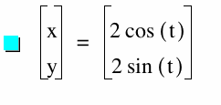
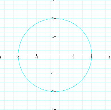
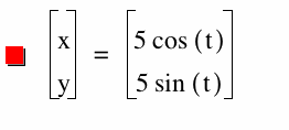
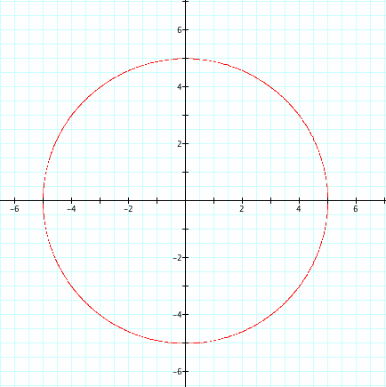
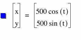
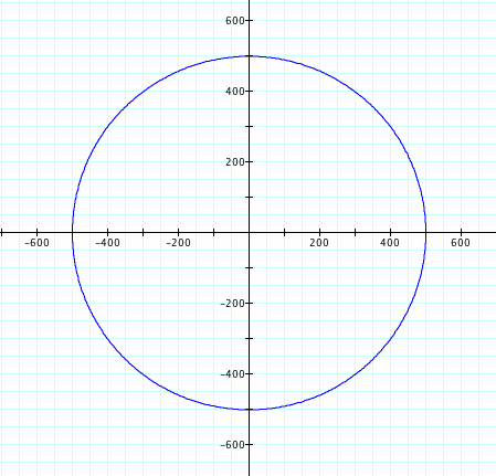
We observe that when a = b no matter if it is a = b = 1, 2, 3, 5, ....50,...or 500 the graph still creates a circle.
So we notice that it is always a circle because if a = b we can always eliminate the parameter t and rewrite the unit circle equation in the form of the equation of a circle (since the equation of a circle is based on the unit circle equation with a radius 1).
Consider: a = b = r

If a = b we can always factor out a common factor. Thus getting the equation of a circle each time with radius 1 and center (0, 0).
For the second investigation we will look at the graph when a < b. In this problem we will substitute different values in for a and b: a = 2 and b = 5.
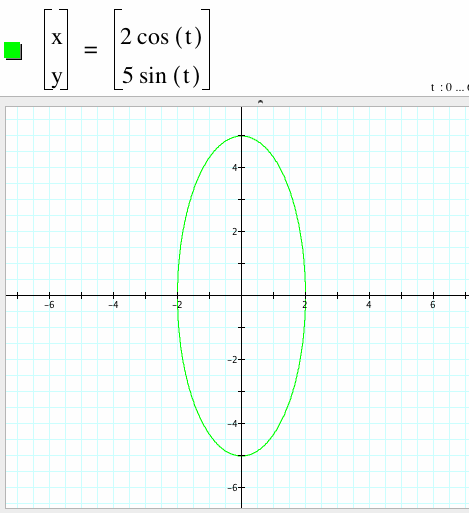
We notice that our graph is no longer a circle but has been stretched vertically. So we notice that we get an ellipse as opposed to a circle. Also we observe that our y-intercepts have changed, now they are (0, 5) and (0, -5). But our x-intercepts from the original graph where a = b = 2 did not change.
For the third graph we will look at what happens when a > b. In this problem we will use a = 5 and b = 2 this time.
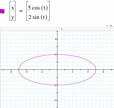
Observe that this also creates a graph that is not a circle. This graph have been stretched horizontally. We see that our y-intercepts are the exactly the same as they were in the graph of a = b = 2. However, our x-intercepts have changed they are now (5, 0) and (-5, 0).
We notice that when we vary the coefficients of sint and cost, the shape of the graph becomes an ellipse. We also suspect something else. We observe that it seems as if the coefficients of the sint and the cost are the x-intercepts and y-intercepts of the ellipse. However, let us try one more example to see.
Let's look at a = 3 and b = 4.
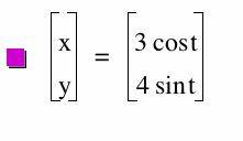
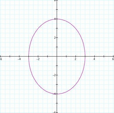
If you would like to experiment with different values of a and b, the graphing calculator file is attached.

For the second investigation let's look at the following parametric equation:
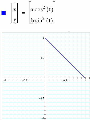
Similar to our first investigation we set a = b = 1. We have a x-intercept at (1, 0) and a y-intercept (0, 1). We notice that the graph results in a straight line that connects the 2 intercepts. We see that the graph has stretched slightly vertically. Notice that this function only has values in the first quadrant. Since the cosine and sine functions are being squared then the values are always positive. We do not have any negative intercepts because the cosine and sine equations are both being squared (as long as we keep a and b positive).
Now let's look at the graph when a < b. Let a = 1 and b = 5.
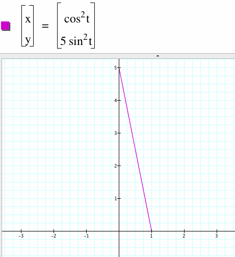
Adding the coefficient of 5 allows the graph to vary from 0 to 5 while still only having positive values in the range (since sine is squared). Furthermore, we see that the x-intercept is the same but the y-intercept has changed to (0, 5).
For the third graph let's look at a>b. In this problem we will use a = 5 and b = 1.
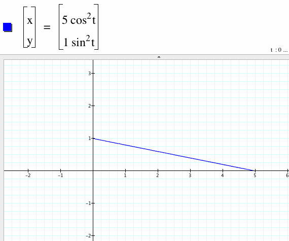
Looking at the graph above, we notice that the graph is a longer line that is stretched horizontally this time. We see that the y-intercept this time is exactly the same as the original graph but the x-intercept has changed to (5, 0). Also, we are still in the first quadrant only.

Now let's look at the following parametric equations:


Consider the following equation when a = b = 1:
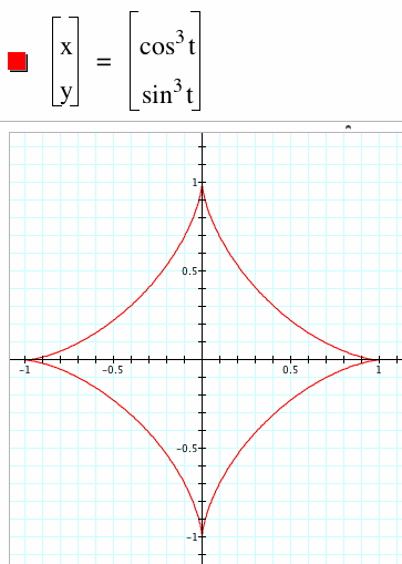
In the graph above we notice we have negative values and positive values again for x and y.
For the second graph we will examine what happens when a < b. In this problem we will substitute a = 1 and b = 4.
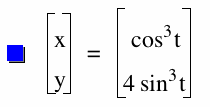
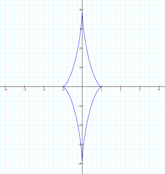
Observe that our graph has been stretched vertically. The x-intercepts stayed the same as our original graph but our y-intercepts changed.
For our third graph let's look at when a > b. Take a = 4 and b = 1 this time.
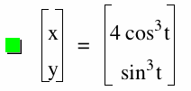
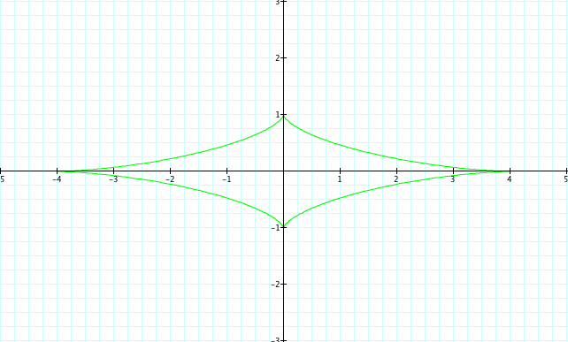
Now we notice the graph has been stretched horizontally.
Click here to explore and enjoy the graphing calculator file when the cosine and sine functions are cubed.
Let's investigate a little further. We will look at what happens when we raise cosine and sine to more odd powers.
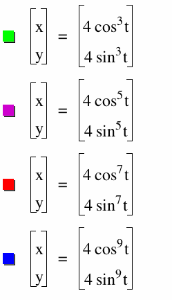
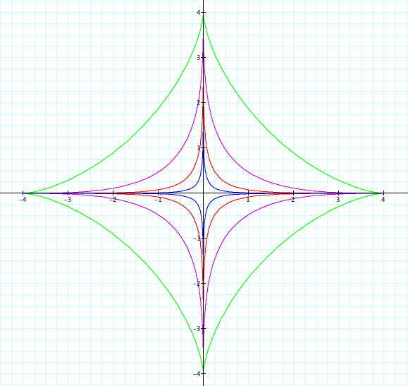
We took positive values for a and b, a = b = 4, and graphed these parametric equations above with different odd powers.
Then we looked at a = b = 4 and graphed these parametric equations below with different even powers.
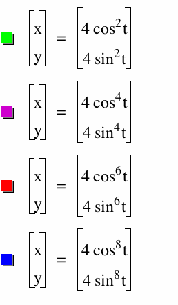
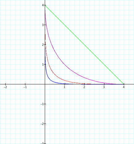
Even if we change a to be negative and b positive (vice versa), we still see some interesting graphs. In conclusion, we have observed a wide range of curves that are all produced by sine and cosine both singly and in parametric pairs. Individually, the curves are continuous but in pairs we observe they are bounded.