
Assignment 10:
Parametric Equations
by Bennett Lewis
In this assignment, we will take a look at different forms of the parametric equations using the graphing calculator application:
Introduction
In order to understand what the graph will look like for this set of parametric equations, let’s review the idea of parametric equations
. A parametric curve consists of two functions on the plane x(t) and y(t). These functions describe the (x,y) coordinate in respect to a parameter t. These equations are widely used in areas of physics for range of motion, trigonometry, and many other areas of mathematics.
For example, let x(t) = t+1 and y(t) = 2t, when t=1, then (x,y)= (2,2) on the cartesian plane. When you set it to an interval like 0 ≤ t ≤ 5, the the graph looks like the one below.
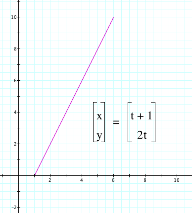
Here we have a line on the interval 0 ≤ t ≤ 5. We could rewrite these equations as one linear equation. In order to do so, we must find the slope and the y-intercept. To find the slope, let’s take the two points (1, 0) and (2,2). Calculating the change in y over the change in x will give us our result. In this case, the slope is 2.
So for our linear equation, we have y = 2x + b. To find b we must simply choose one of our points and and plug in the known values. Let’s use the point (1,0):
y = 2x + b
0 = 2(1) + b
0 = 2 + b
b = -2
Therefore, the linear equation that represents this parametric equation is
y = 2x - 2
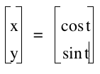
Now, let’s explore our original parametric equations: x = cos t y = sin t What do you expect to see on the graph for these two functions? Consider the interval 0 ≤ t ≤ 2π. For the following values we get:
t=0, x = cos 0 = 1; y = sin 0 = 0; (1, 0)
t= π/2, x = cos(π/2) = 0; y = sin(π/2) = 1; (0,1)
t= π, x = cos(π) = -1, y = sin(π) = 0; (-1,0)
t= 3π/2, x = cos(3π/2) = 0, y = sin(3π/2) = -1; (0,-1)
t= 2π, x = cos(2π) = 1, y = sin(2π) = 0; (1,0)
These coordinates look very similar to the coordinates of the unit circle. Now let’s look at the graph.
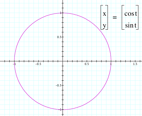
Notice that the graph is identical to that of the unit circle. Therefore, using this set of parametric equations can help us generate various coordinates on the unit circle. What will happen to the graph if the x and y functions are switched around?
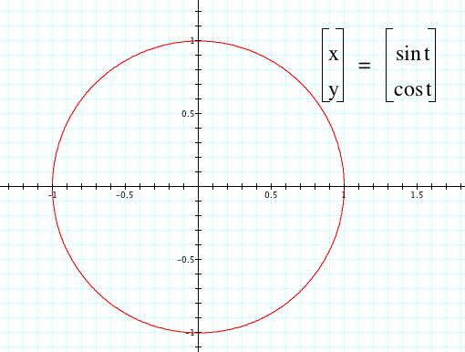
It still remains the same graph for this standard interval. Now let’s take a look at various forms of this equation. What if we changed the form of x(t) to x(t) = cos(at)?
Here we have in red, the original graph, and in purple, the altered graph of x(t) for 0 ≤ t ≤ 2π. Instead of having a full completion of a circle, the graph resembles a rotated parabola. Even if we changed our interval and increased the end boundary of the interval, the graph would not change shape.

When we start to manipulate y(t) also, we start to notice the main shapes and curves that can be formed from increasing, a, b in
x(t) = cos(at)
y(t) = sin(bt)
When the values of these a and b are changed, the numbers of curves and spirals increase.
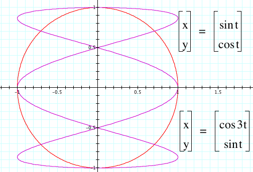
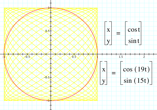
In red, we can see the original graph. In purple, we can see how x(t) is affected by the parameter a for x(t) = cos(at). In yellow, we can see how y(t) is affected by the parameter b for y(t) = sin(bt). As a and b increase, the number of curves and spirals increase as well. For the yellow equation, the curve is shifting and increasing in respect to the “x-axis” on a cartesian plane which makes sense since x(t) is the function with the parameter. For the red equation, the curve is shifting and increasing in respect to the y-axis which follows from the fact that y(t) is the function with the parameter.
Now let’s investigate the effect of the original parametric equation when we change it to the form:
x(t) = a cos(t)
y(t) = b sin(t)
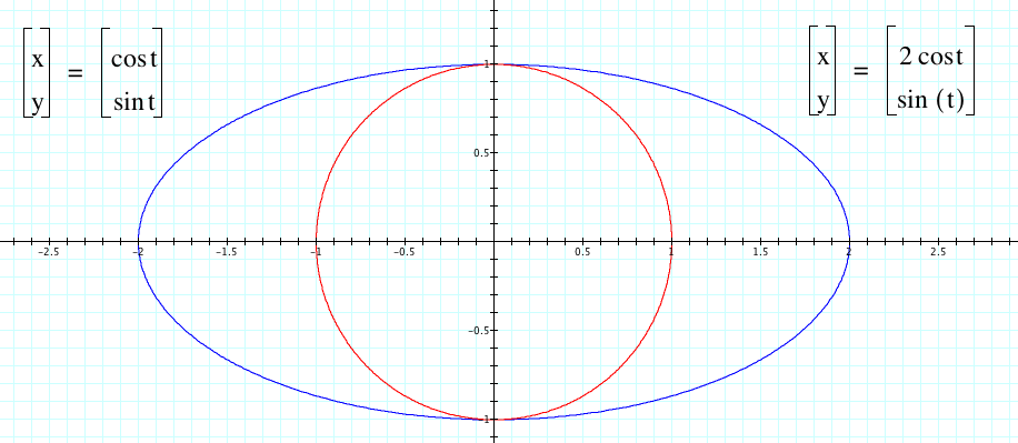
Take a look at the following graph where blue represents the original and red represents the graph of x(t) when a=2. Now take a look at the graph when b = 2.
Now take a look at the graph when b = 2.
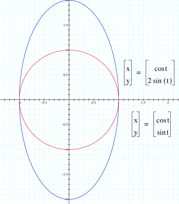
Now take a look at the graph when b = 2. Instead of the curve being stretched with respect to the x-axis, the curve is stretches in respect to the y-axis. So, as a increases, the curve stretches horizontally on the x-axis, which corresponded to the fact that x(t) is altered. Also, as b increases, the curve stretches vertically on the y-axis, which correlates to the fact that y(t) is altered.
Check out a video of a and b changing to see what happens as a and b increase.
You can see more about these equations using the Graphing Calculator application.