
Assignment
2: Comparing y = 2x2 + 3x - 1
and y = 2x2
+ 3x - 1 + xy
Goal: Compare the graphs of![]() and
and ![]()
![]()
When first graphing both equations we get the
following:
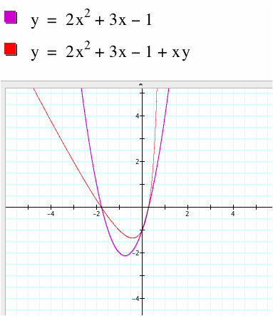
Some initial observations include the obvious
differences between the two graphs. Clearly the first equation is what we
would expect, a normal parabola. The second equation seems to have the
same basic properties of a parabola (same end behavior, a minimum point),, but appears to be skewed in some way.
Zooming out, however, a different picture
emerges.
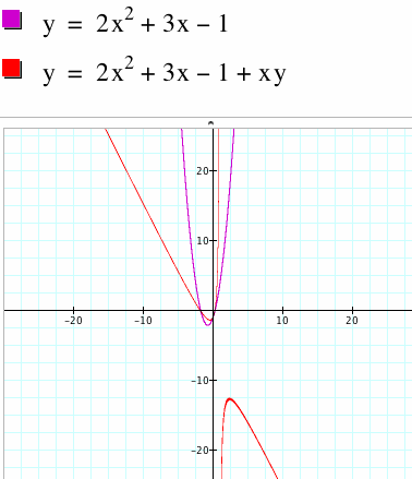
This picture presents a much different
scenario. Now we see that there is another part to the graph. We can
also infer that there is likely both a vertical asymptote but also an oblique
asymptote. Clearly there is more going on here then meets the eye.
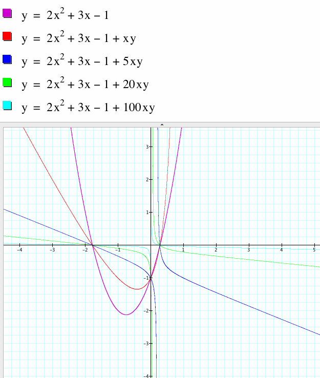
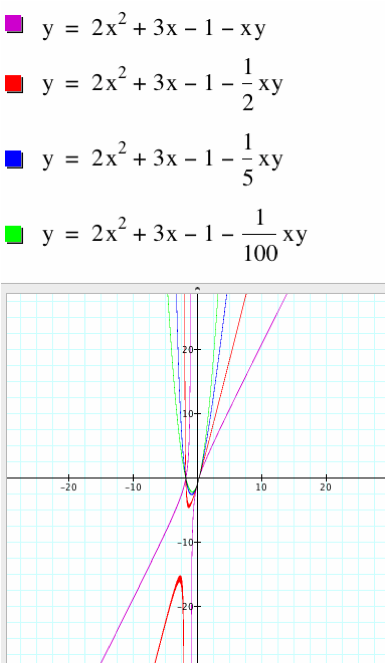
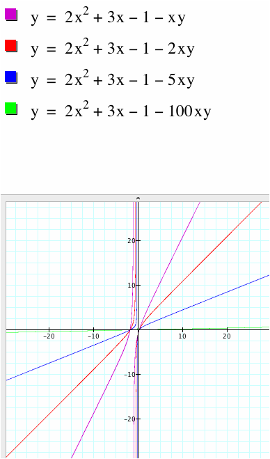
As we increase the coefficient of xy, we see that the minimuma and
maximum get closer and closer, almost touching by the time we have gotten to n
= 20. The vertical asymptote seems to be staying relatively still, but
the slope of the oblique asymptote seems to be approaching 0. I would
guess for n very large the graph would mimic the graph of![]() , where C is some
constant. This makes sense as for large n the y, x-squared, x and
, where C is some
constant. This makes sense as for large n the y, x-squared, x and
constant term all serve as a constant term and we get C = xy, or ![]() .
.
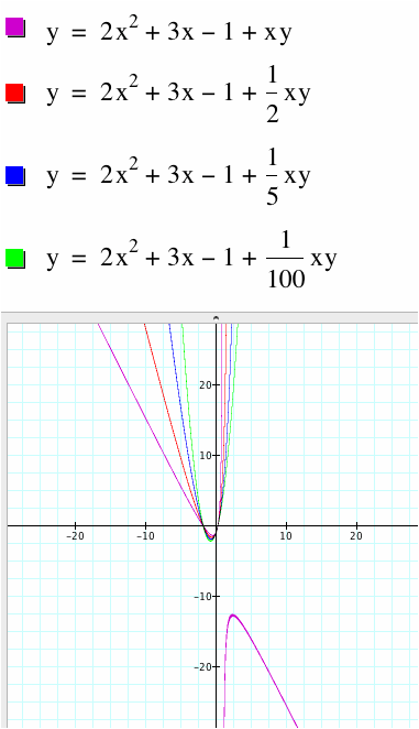
If we decrease the coefficient of xy towards 0, we see that the graph gets closer and closer
to our original parabola. This makes sense as we are minimizing the
effect of the extra xy term. If xy = 0, then we
would simply have the same graph we started with.
When the coefficient becomes negative but from
0 to -1, we see that the graphs are very similar to the reflections over the
y-axis of the graphs above. At first the graphs are very similar to the
parabola itself, but then the graph splits.
Finally as we make the coefficient more
negative we see that again we have reflections over the y-axis of the original
coefficients of the same absolute value.
The animation of![]() and
and![]() below gives a good visual representation of how as n
gets closer to 0 the graph of
below gives a good visual representation of how as n
gets closer to 0 the graph of
![]() approaches
the graph of
approaches
the graph of ![]() and as n gets larger the graph eventually appears to
separate and eventually begin to approach
and as n gets larger the graph eventually appears to
separate and eventually begin to approach![]() .
.
An interesting observation that can be made using the graph above is the location of the roots in both equations. It appears that the roots do not changes as the n-value ranges from -10 to 10. The animation below is a zoomed version of the one above, focusing on the roots of the equations.
This is logical as the roots exists where y = 0. If we plug y = 0 into both equations, you see that we end up with the same quadratic function to solve, which results in identical roots.
In the case we are working with, the graphs will always be either a parabola or a hyperbola. However, if we include a y-squared term, things may change. This is due to the rules concerning the discriminant of a non-degenerate conic. A conic takes the general form:
![]()
If the discriminant (![]() ) is equal to 0, the equation is a parabola, if the discriminant is greater than 0, it is a hyperbola, and if it is less than zero, it is an ellipse.
) is equal to 0, the equation is a parabola, if the discriminant is greater than 0, it is a hyperbola, and if it is less than zero, it is an ellipse.
In our original case, A = 2, C = 0, and B varied. However, since B is squared, the value of the discriminant is always zero or a positive number. Hence, when B = 0, we have the parabola, but when B does not equal 0, we have a hyperbola. That is, the only time our original equation with the xy term will be a parabola is precisely when the coefficient of the xy term is 0.
This leads to the fact that an equation an like:
![]()
can give us any type of conic, depending on n. If n = 0, we have a circle. If -4 < n < 4, but n does not equal zero, then we have an ellipse. If n = 4 or n = -4, we have a parabola, and if n > 4 or n < - 4, then we have a hyperbola. The video below exhibits these relationships.