---

Rational Function Study

By: Amanda Sawyer

We will study the formula:

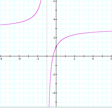
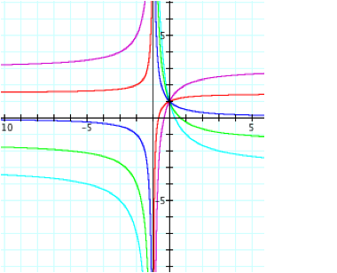
To study this equation, let us look at three separate situations. When we allow a = 3 and all other valuables to equal one, we get the following graph.

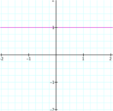
When we allow all values to equal one, the equation becomes y = 1 and we get the following graph.

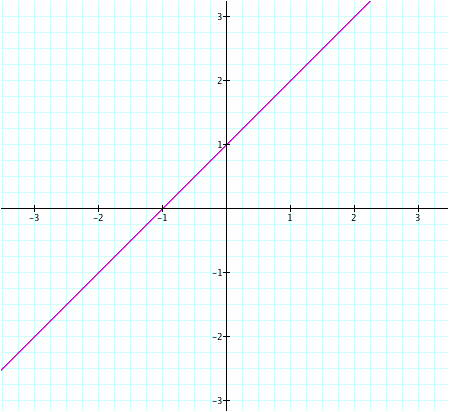
When we allow value of c = 0 and all other values are one, the equation becomes a polynomial, and we can see this in the following graph.

From the equation and its graph, we can clearly see that it can be either a rational function, a polynomial, or the function y = constant. To study this function, we will look at its vertical asymptote, horizontal, asymptote, slant asymptote, domain, range, areas of increasing and decreasing, areas of concavity, x-intercepts, and y-intercepts. First let’s look for the asymptotes.

1) Vertical Asymptote

To find the vertical asymptote, we first need to simplify the equation and then set the denominator equal to zero. This value will become the vertical asymptote. If we assume that the numerator is not a multiple of the denominator, then the vertical asymptote will be:

Otherwise, we don’t have a vertical asymptote, and our graph is a straight line or a polynomial. We can observe this behavior in the animation below where the value of c is varied from -5 to 5. In the graph below you will see the vertical asymptote in red from the equation above and the general function in purple.

2) Horizontal Asymptote and Slant Asymptotes

If a or c are not equal to 0, we will always have the same degree on our numerator as well as our denominator. This allows us to easily calculate the Horizontal Asymptote. We find this value by taking the ratio of the leading coefficient of our numerator and denominator. Our leading coefficient of our numerator is a and the leading coefficient of our denominator is c, thus the horizontal asymptote is:

If c = 0, we know that our graph is a polynomial, and it does not have any asymptotes. If a = 0, we know that our horizonal asymptote is y = 0.

Since the degree of your numerator will always be the same as our denominator, we will not have a slant asymptote.

In the graph below you will see the horizontal asymptote in red from the equation above and the general function in purple.

This helps to determine our graphs Domain and Range.

3) Domain

If we assume that the numerator is not a multiple of the denominator or c not equal to 0, then graph has a vertical asymptote. From that information we can find the intervals for which our domain exist by excluding those points. Therefore we can define the interval to be:

Otherwise, our graph will have a domain of all real numbers.

4) Range

We can also determine the range of our graphs since we defined our horizontal asymptote. When the numerator is a multiple of the denominator or c is not equal to 0, its range will be equal to the single value of the multiple. Yet, if that situation does not occur, we can find the range using its vertical asymptote. This equation gives us the range of:

Next let’s study when our graph is increases and decreases:

5) Areas of Increasing and Decreasing

We were taught in calculus, that we could determine when a graph increases and decreases by taking the derivative of our function. The derivative of our function is:

We can tell from this derivative that our whole function will be increasing when our numerator is positive, and our whole function will be decreasing when our numerator is less than 0. When the numerator is equal to zero, we have two different cases:

1) a = c and d = b or a = b and c = d, then we will have a straight line.

2) If , the graph is increasing.

3) If , the graph is decreasing.

This can be observed in the graphs below.

Equations	Graph

Now let’s study the concavity of our function:

6) Areas of Concavity

We can determine the concavity of our function using the second derivative. When the values are positive in our second derivative, the graph is concave up. When the values are negative in our second derivative, the graph is concaved down. Our second derivatives is:

This gives us different cases where our graph is concave up and concave down.

If

a) for some value of x such that then our graph is concave down.

b) for some value of x such that then our graph is concave up.

If

a) for some value of x such that then our graph is concave up.

b) for some value of x such that then our graph is concave down.

Now, let’s investigate what happens to our x-intercepts and y-intercepts.

7) X-Intercept

When our function simplifies to a constant, then it does not have an x-intercept. Otherwise, the graph has an x-intercept when its numerator is equal to 0. We can find this value by setting the numerator equal to zero and solving for its variable:

In the graph below you will see the x-intercept represented as the line in red from the equation above and the general function in purple.

8) Y-Intercept

We can find they y-intercept for any of the functions by setting my x values equal to 0 and solving.

This value gives us the y-intercept.

We have now been able to explore this equation and each of its parts using Graphing Calculator. Through the use of its utilities, we are able to show how each of our original graphs relates to its different elements. This tool makes it easier to check our solutions without having to manually create each of our equations.

---

Return to Homepage