
Making Money with Spreadsheets
An Exploration of Excel Spreadsheets
by
Sarah Major
In this ever-changing world in which technology reigns supreme, acquiring the latest and most innovative forms of technology is of vital importance to any business or organization. Therefore, the analysis of different technological investments is a serious endeavor that should be carefully done. Specifically, one of the main forms of technology that has the biggest effect on whether a business is successful or not are those dealing with information systems. These are all of the hardware and software businesses use to collect, store, and transfer data.
When choosing a new form of information systems technology, a business looks for forms that will return as large of a profit in as small of an amount of time as possible. To predict this, businesses calculate ROI, or return on investment. This calculation is the percentage of additional profits produced because of an investment in a certain form of information systems technology. The most worthwhile investment will produce not only a positive ROI in the least amount of time possible but also the highest ROI based on a predetermined period of time. Therefore, the analysis of this calculation in regards to different investments can assist in choosing the most profitable investment opportunity and prevent spending more money than necessary.
With this in mind, for this write-up, I am posing as the CIO (chief information officer) of a developing company, which is looking to invest in new information systems technology. To aid in this investment, I have formed an ROI calculator using Excel. Below is a screen shot of the full calculator (with values already inputted):

By simply adding the inputs of projected cost of capital, initial cost, and estimated annual increase in revenue and net cost savings based on projected economic statistics, estimates of not only net revenue but also of the ROI will be calculated. These values indicate whether the new technology will be a worthwhile investment and how long it will take to produce a worthwhile profit. This ROI Calculator can be a vital tool for any business wishing to invest in new information systems technology or any other form of new technology. By analyzing the ROI calculations or graphs of ROI calculations over time, any business can utilize the data to choose the best and most worthwhile investment that will produce the quickest and greatest profit for the business.
First, I will discuss the top portion of the calculator. Below is a screen shot of this portion:
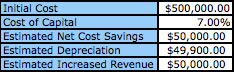
This portion of the calculator contains all of the inputs required for the ROI calculations. The first input, initial cost, is the total cost of the new technology at the time of purchase. The second input is the cost of capital, which is the percentage of the initial cost that the company will pay back on an annual basis. This is chosen by the business itself in consideration of their payback methods and amount of revenue. This and all of the other calculations besides initial cost are annual estimates.
In the third row is estimated net cost savings. This is how much money the business will save by investing in the new technology and is based on its efficiency and productivity. The higher the efficiency and effectiveness of the new technology, the higher the amount of cost savings will be per year.
The fourth estimate, estimated depreciation, is how much worth the technology uses as it becomes older and more outdated. What makes this estimate unique is that Excel has a predetermined formula to calculate it. One simply types “=SLN(cost, salvage, life)” with the corresponding estimates of the three items. “Cost” corresponds to the initial cost of the technology, so the corresponding cell can be referenced in the formula. “Salvage” refers to the salvage value of the technology after its useful life, and “life” is how long the technology is estimated to be useful and beneficial to the company or organization. In essence, this is how long the company intends to use the technology before purchasing a new form to replace it.
The last input is estimated increased revenue. This is the estimated calculation of how much more revenue the company will receive as it grows and develops per year, or how much more profitable the company becomes yearly. This is assuming that the profits grow at the same rate every year. Though this is not logical in a real world setting, this functions as a constant for the purposes of comparing different investments.
Below is a screen shot of the bottom portion of the calculator:
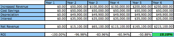
This portion of the calculator contains the yearly estimates for increased revenue, cost savings, depreciation, and interest over a six-year period. I chose this length of time because many businesses believe that if they do not return a profit with the entire initial cost of the technology paid off within this amount of time, the investment was not a worthwhile one. If a company wishes to use a longer length of time, all they need to do is select an entire column and drag it across to product the formulas in as many more columns as they would like.
The only estimates inputted manually are contained in the first year, since the only monetary exchange occurring during this year is the actually initial cost. The rest of the entries use formulas to produce their values.
In this first row, increased revenue is calculated by adding the estimated increased revenue inputted in the top portion of the calculator to the previous year’s increased revenue. This is because the technological investment is expected to produce an increasing amount of revenue at this manually inputted rate.
The cost savings entries are simply the corresponding estimate from the top of the calculator each year, as is depreciation. This is because they are based on the same yearly estimate each consecutive year and do not change as the years progress. Interest, however, is the cost of capital percentage multiplied by the initial cost. This calculation is how much interest will be charged to the company until the whole cost of the investment is paid off. Depending on how the money is obtained, the formulas within these cells may have to be changed. Some interest is charge on the initial balance while others are charged on how much of the intial balance is remaining after portions have been paid. For the sake of this analysis, I have chosen for interest to be charged on the initial balance each year.
The next line contains total revenue for each year. This is found by subtracting the sum of depreciation and interest from the sum of increased revenue and cost savings. In essence, this is how much in the positive the company comes out each year.
The last line is the calculated ROI. This is found by subtracting the initial cost from the total revenue and then dividing by the initial cost for each year. A negative calculation occurs when the business has not acquired enough cumulative revenue to make up for and pay off the initial cost. Once the company has done so, a positive ROI occurs. Using conditional formatting, I caused the cell to turn green when a positive ROI is achieved. This makes it easier to see which investment produces a positive ROI first when looking at a series of investments.
If one wishes to use the ROI calculator, he/she should simply change the values in the input table, which is the first table on the spreadsheet, and the following tables will conform to the given inputs. To compare a series of investments, simply copy and paste the entire calculator, making sure the formulas are also carried over into the copied version.
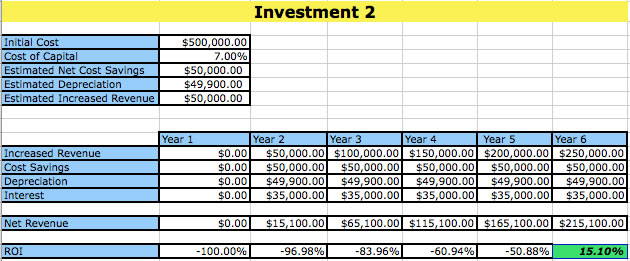
In the screen shot of the entire calculator, I inputted some values in the top portion of the calculator to simulate a theoretical application. Below is the screen shot again:
In this example, the initial cost of $500,000 was inputted into the first slot of the spreadsheet, the cost of capital of 7%, estimated net cost savings of $50,000, and estimated increased revenue of $50,000. The estimated depreciation was calculated by using the SLN function and inputting $500,000 for the cost, $1,000 for the salvage value, and 10 years for the useful life. These values calculated an estimated annual depreciation of $49,900, which makes sense when analyzing the values used to acquire it. The salvage value refers to what the technology will be worth after the useful life of ten years. If the value of the technology decreased at the same rate annually and ended with this salvage value, it would have to decrease by $49,900 to get $1,000 after ten years.
After these values were inputted into the spreadsheet, the total annual net revenue for the next six years was calculated. This value increased by $50,000 each year after the initial year, which makes sense that all of the values were the same except the increased revenue that increased by $50,000 each year. In the last row of the calculator, the ROI was produced. Between the first and fifth years, each year produced a negative value, which makes sense because adding the total revenue produced a value less than the initial cost. Only during the sixth year did the total revenue for the whole six years produce a value greater than $500,000. The conditional formatting also flagged this positive value.
To extend the application of this calculator, I have also chosen to include a comparison of five fictional investments to see how the calculator can aid in choosing the best option. Below are screen shots of each investment:

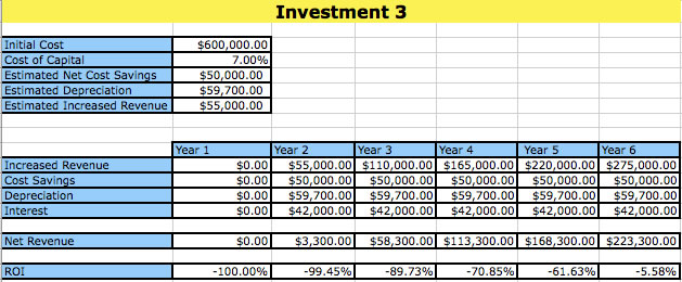
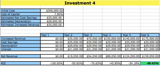
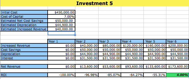
Because of the conditional formatting, we can see which investments produced a positive ROI after the six year time period. Therefore, investment 3 can be eliminated because it did not return a positive ROI. Of the others, we can see that investment 4 produced the greatest ROI for this time period, and thus, we would want to choose this technology instead of any of the others.
We can also prompt Excel to produce a line graph of the ROI calculations to visually see which investment would be better and how the ROI calculations compare over time. Below is a graph of the above five investments:

As the graph displays, we can see that a majority of the investments produce similar ROI calculations. However, the purple graph, which is investment 4, greatly outperforms the rest. We can therefore safely choose this as our best investment.