Investigation I

The statndard form of a parabola is

where a, b, c and x are variables in the equation that can be changed to change the shape and translate the graph in the coordinate plane. Each time any value of these variables is changed, the roots of the eqaution is also changed, hence where the graph crosses the x-axis is different. For example, lets begin with a function where the variable b is different and lets explore what this means in terms of roots.

(black)

(gray)

(light blue)

(purple)

(red)

(dark blue)

(green)

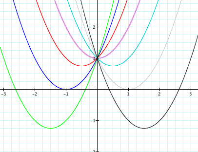
By studying the graph above, you will notice that therea are no real roots for -2 < b < 2. Here for b = -2, then the eqaution is tangent to the x-axis and thus has one real positive root. When b < -2 graph falls below the x-axis and thus has two real positive roots. Likewise, when b = 2, the graph is tangent to the x-axis and thus has one real negative root and b > 2 falls below the x-axis and has two real roots.

Now lets explore the vertices of these parabolas. If we wanted to connect each vertice with a curve, we would begin by looking at whether it would be concave down or concave up. By the graph we can recognize that the curve must be concave down since the parabolas seem to be falling below the x-axis the farther b gets from 0. Noext we should look at the maximum of the new curve which is the point where it touches the greatest vertice in terms of the ordinate. Since the largest value of y in each vertice is 1, then the maximum of the new curve must be 1. This is the point where it intersects with the equation where b = 0. If we choose two points that the curve must pass through, say vertices (1,0) and (0,1), then we can find an eqaution that is negative, has a maximum at y = 1 and passes through the points (1,0 ) and (0,1). Therefore the eqaution of the curve fitting these conditions is

which happens to be the opposite of our original eqaution

Therefore the new graph looks like

We can genralize this by stating that whenever you begin with a basic equation for a parabola where you only change the value of b, holding all else constant, to find the curve that passes through every vertice that can be created with the conditions above, just take the opposite sign of the original equation to find that curve.

Now lets look at the equation

and lets graph it in the xb plane as shown:

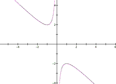
Next if we overlay an equation of a parallel line to the x-axis, specifically

we get a line that intersects the graph in two points. From this we can see that where this line intersects the graph in the xb plane are the points for roots of the original equation.

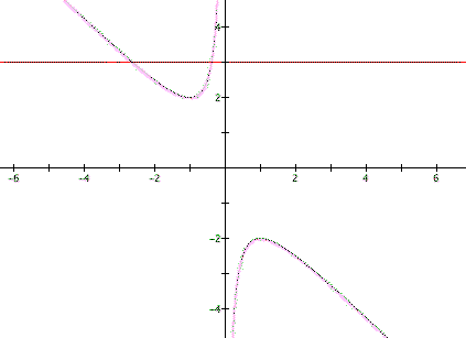
It is clear on a single graph that we get two negative real roots of the original equation when b > 2, one negative real root when b = 2, no real roots for -2 < b < 2, One positive real root when b = -2, and two positive real roots when b < -2. Now lets explore the equation when c = -1,

and we will use this equation to overlay the previous graph:

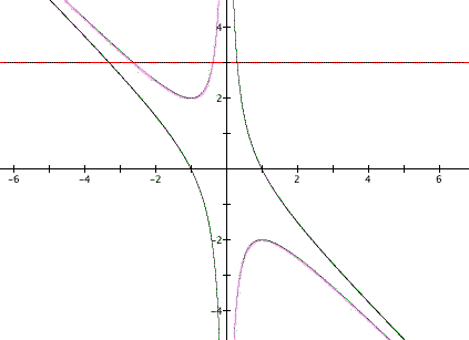
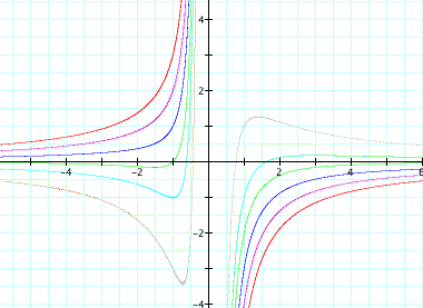
Similarly to the last equation, wherever the graph intersects the parallel line is considered to be the roots of the original equation for that particular value of b. Hence the same true in this case except that there is always one real negative root and one real positive root for any value of b. So we see that when c is negative there are two real roots, one negative and one positive, and when c is positive there are two roots but their signs differ depending on the value of b. Below is a graph that shows different values of c where b = 3 so that we can understand that becuase of the shape of the graph of each particular equation, we get different roots for b.

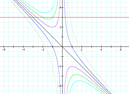
Notice that when c = 0, the graph is just the equation of a line through the origin. Now lets explore the equation

by overlaying it on the previous graph and look at its relation to the quadratic formula.

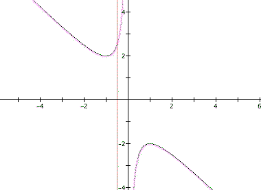
As we can see the graph of the new equation is a vertical line which only passes through one point of the quadratic equation, never two points and never both parabolas. Now lets consider the graphs in the xc plane.

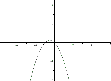
The quadratic equation is a simple concave down parabola that moves its vertice depending on the variable for b while the line the we constructed earlier still intersects teh parabola at its vertice. Below is a universal graph of a few values of b from [-3,3].

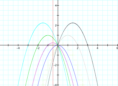
Lets assume that we want a curve to intersect all vertices of the parabolas no matter the value of b. By comparing this to an earlier graph above, it looks as though the opposite curve would work for this group of parabolas than it did in the beginning. Hence my assumption is that the standard equation for a parabola, concave up, will satisfy these constraints.

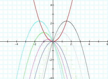
Now if we graph these equations in the xa plane, the graph of those functions looks like:

Now if we take the values of b from [-3,3] we get a system of graph like this:

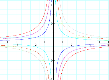
As we can see if b is negative then the graph lies in the first and thrid quadrants but if b is positive then it lies in the second and fourth quadrants. We can also see that there is not a single curve that will intersect every vertice of these parabolas but maybe two lines through the origin with opposite slopes, -1 and 1, might fill these consraints.

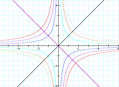
Now lets explore the the roots of the equation

in the xa, xb, xc and xd planes. This time lets graph the equation in all planes overlaying each other where blue is xa, purple is xb, red is xc and green is xd.

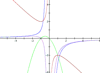
As you can see that as previously explored, a horizontal line will give you the two roots in the xc plane, which was previously the xb plane, a vertical line will give the roots of the parabola in the xd plane, previously xc plane. Now lets take a closer look at the xa and xb planes.