
Inside Out:
Parametric Curves
by
Christa Marie Nathe
A
parametric curve in a plane is the set of functions where x = f (t) and y = g (t). Random or arbitrary values called parameters determine the values for
x and y. When we think of a function to be plotted on the x-y
coordinate plane, the value for x
determines the value for y.
However, if we are given a complicated function where it is difficult to
separate x from y, then it will be very difficult to represent the
function graphically. However, by
transforming the function or expression into parametric form we can derive a
graph for the desired expression based on random values which we will here on
refer to as the variable t.
Take for example the function y = x2 which we can be parameterized by equating x = t and y = t2 which yields a function expressed in terms of the
parameter t. In essence, we are graphing functions
and expressions from the inside out, instead of directly through x and y.
We will be observing several sets of curves based on
the following:
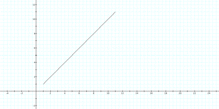
x = a + t
y = b + kt
The graph below is based on 1 being the values for a, b, and k
where the range for t is from 0-10
The following graph represents where the value for a
= -1 where all other values remain at
1 and the range of t from 0-10
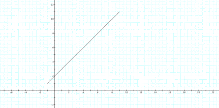
How has the graph changed? Instead of the curve
beginning at (1,1), changing the value of a to -1, changed the initial point to (-1,1).
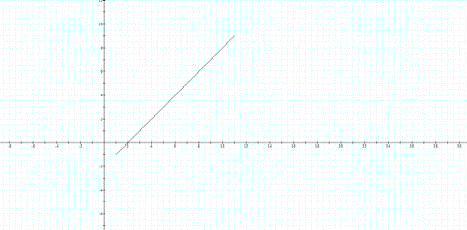
The next graph reflects the change in value where b
= -1 and the other values remain at
1, t from 0-10. As you compare
this graph to the first, you can see that changing b from 1 to -1 means altering the initial point from
(1,1) to (1,-1).
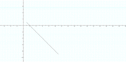
Finally, by making k = -1, where a and b are set at the
value of 1, and t from 0-10 we can
see that the slope of the line is no longer positive, but negative.
How does the range of t affect the graphs? The value for t is set between zero and ten, for the previous graphs.
This means that the graphs you observe only reflect the parametric equations
along this scope. If the range were increased, or decreased that would directly
change the size of the parametric graph.
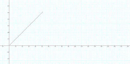
In the following graph the range of t has been changed from 0-10 to 0-50 where a, b, and k all have a value of 1. Here we made the graph smaller since the curve is longer
when its range is increased.
Now that we have observed how each of the variables a, b, and k shape the graph of the curve, we can make some
conjectures based on these examinations to determine various other graphs.
How will the graph look if the value for k is increased while values for a and b
remain constant?
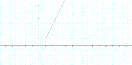
Graph 1: a
= 1, b = 1 and k = 2
The slope of the curve has become more steep than when
k = 1
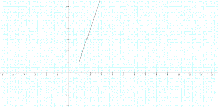
Graph 2: a
= 1, b = 1 and k = 3
This curve is becoming more vertical as the value for k increases.
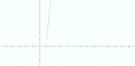
Graph
3: a = 1, b = 1 and k =
10
For a little excitement, lets make a k larger than the in the previous examples to show that
the slope is becoming more steep as k
increases.
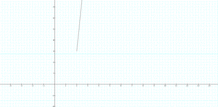
Graph 4: a
= 2, b =3, and k =10
Here we are setting the range of t from 0-10, where
now we know from experience that the scope of t affects the length of the
curve.
In this graph we are testing our knowledge about how
the values of a, b and k serve to direct the curve.
Where does the curve begin? (2,3)
This confirms our previous study of examples above.
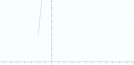
Graph 5: a
= -2, b = 4 and k = 10
Again, as expected the graph has an initial starting
position at (-2,4) and continues with a positive slope as we have set for the
value of k.
From this investigation we have learned that
parametric equations are based on a range determined by the scope of t, and from there an equation can be represented
graphically without being limited to exclusively using x to determine y or y to determine x.