Parametric Equations
by Michael Walliser
Consider the following set of parametric equations:
x = a + t
y = b + kt
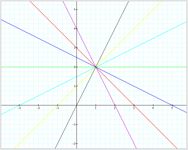
Let's see what happens when we graph these equations with varying values of a, b, and k. We'll start by holding a and b constant, let's say at a = 1 and b = 2, and using k values of -2, -1, -1/2, 0, 1/2, 1, and 2.
![]()
k = -2 ______ k = -1 ______ k = -1/2 ______ k = 0 ______ k = 1/2 ______ k = 1 ________ k = 2

We see that k simply represents the slope of the curve. This makes sense when we consider that, for any change in t, y changes at k times the rate that x changes. Be aware that if we multiply t by a coefficient in the x equation, then the slope will be the ratio of k to that coefficient. Notice also that all the curves pass through the point (1,2). This point is common to all the curves when t = 0, so unsurprisingly, it can be represented more generally as (a,b). Let's check this hypothesis by varying the values of a and b.
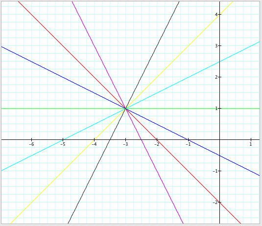
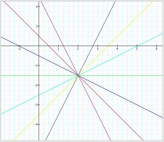
The following graphs uses the same k values, but we now set a = -3 and b = 1 in the graph on the left, and a = 2 and b = -1.5 in the graph on the right.
![]()
k = -2 ______ k = -1 ______ k = -1/2 ______ k = 0 ______ k = 1/2 ______ k = 1 ________ k = 2


Indeed, the slopes stay the same, and the curves are concurrent at (a,b) in each graph.
If we want to model these graphs using y as a function of x, we can simply solve the x equation for t, then plug the solution into the y equation. For instance, we can rearrange x = a + t to say that t = x - a. Thus, we can rewrite y = b + kt as y = b + k(x - a), or y = kx + (b - ka), where k is the slope and b - ka is the y-intercept. If we observe our graphs above, we see that these slope-intercept equations hold for all values of k, a, and b.