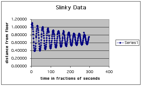
The situation: A slinky was held above a CBL probe that had been placed on the floor. When the lower end of the slinky was released it bobbed up and down, and the probe measured the distance from the floor 295 times in about 30 seconds. The resulting data is graphed below.

The questions:
Building a model:
Describing the graph verbally helps when starting to search for a model. Clearly the data is sinusoidal, but the waves gradually attenuate, which indicates some kind of decay is happening.
I began my search for a model by considering products of y = sin(bx) and y = e^(-dx). In the graph shown below, b = 10 and d = 0.5.
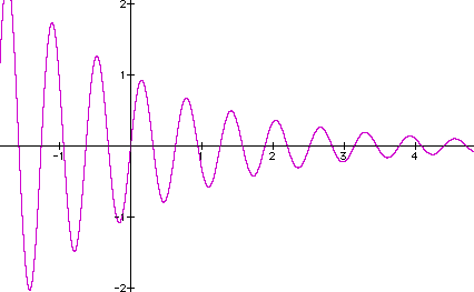
Products of sine and the exponential decay functions thus appear to produce the type of graph needed, although the function above is a long way from becoming a good model for the spring data. The multiplication of the exponential causes the sine graph to be "squeezed" between two boundary curves, y = e^-0.5x and y = - e^-0.5x, as shown by the red graphs below:
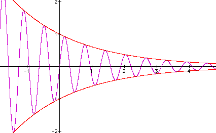
I then began to consider several factors in modifying this function, y = sin(bx)*e^(- dx) to produce a good model.
(1) I noted that the scale requires approximately 3.5 periods of oscillation between x = 0 and x = 100. This aspect of the data required a drastic change in my values for b! Namely, I had to try much lower values of b in order to produce a relatively small number of periods for a relatively large stretch of the domain. b = 0.233 has been my best guess so far.
(2) The horizontal symmetry line of the data is clearly not the x-axis. Therefore, the function would have to be modified to y = sin(bx)*e^(-dx) + f in order to produce a good model. y = 0.72 appears to be a fairly good estimate of the horizontal symmetry line of the data, so I have used f = 0.72.
(3) I had to estimate the decay rate of the exponential function, which is quite gradual. This aspect of building the model was tricky, and I admit to experimenting as well as modifying the model until I had something that seemed to fit well. The best value of d that I have found is d = 0.0039, but I found this value in conjunction with...
(4) modifying the model further. That is, I began to realize that y = sin(bx)*e^(- dx) + f was limited and not providing a good enough fit. I changed the model by adding parameters a, c, and g:
y = a*sin(bx + c)*e^(- dx) + f + gx. The values a = 0.36, c = 0.3, and g = - 0.0002 seemed to help adjust the fit.
Here is a view of my best model so far, although I think there is room for improvement. The blue represents the original data; the purple is the graph of y = 0.36*sin(0.233x+0.3)*e^(-0.0039x) + 0.72 + -0.0002x.
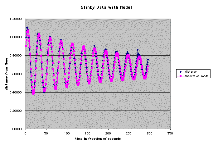
Download this Excel file to see the actual data and model.
A Brief Analysis of the Fit of the Model:
To judge the fit of the model, I calculated residuals, squared them, and found the average. While this calculation is not strictly a standard deviation, it can be used as a comparison when trying different parameters in the model. Obviously, we'd like for the residuals (the difference between the predicted values from the model and the actual data values) to be as small as possible. (Residuals of zero would indicate a perfect fit.)
For the model above, the average squared residual is 0.0025.
But lo and behold, as I experimented I found that adjusting the b-value to 0.235 produces a slightly lower average squared residual of 0.00089. Still I am not completely satisfied with the fit of the model near the end of the data, because the maxima in the model do not appear to match the last two or three maximum values of the data. Further tinkering may be able to lower the average squared residual further and produce a better visual fit.
A plot of the residuals confirms the fact that more tinkering may be needed.
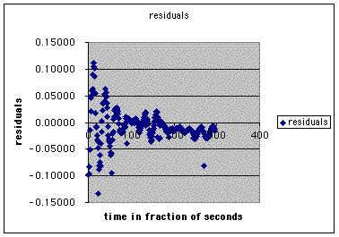
When residuals show a specific trend (e.g., as in the funnel-shape above), it may indicate that the model is not a good fit. However, the close clustering around zero after t = 100 is a relatively good sign. The fact that residuals become all negative toward the end of the time values reflects my visual criticism of the model--that the theoretical values consistently fall below the actual data values.
Interpreting with the Model:
How would the model be useful? And what are its limitations? Obviously, we create models to be able to understand a certain situation better and to make predictions. With this model we may be able to predict the motion of this specific slinky at a later point in time.
However, the main use of this model seems to be in analyzing the type of motion produced by the slinky. The problems I had with fitting the model to the later data values might indicate that the frequency of the motion decreases slightly over time (i.e. the graph "spreads out"). Thus one of the main limitations of this model may be that it does not accommodate such changes in frequency.
On a similar note, the decay rate of the motion may not be constant over time, and might indicate another inadequacy in this model. Perhaps in fact two different models might be needed to capture the data in a piece-wise fashion.
Perhaps the most immediate utility of this model lies in making me think about how to create it! Although I have just begun to explore (the creation of additional parameters a, c, and g was, in particular, not very scientific), I feel that I have started to better understand both the motion and the behavior of a product of sine and exponential functions.