
In this write-up, I investigated a set of data using a Microsoft Excel spreadsheet. First, I entered the raw data into the spreadsheet and graphed the data set. Next, I constructed a function that I thought best fit the data, let the spreadsheet calculate the theoretical data from this function, and graphed this new data set. Then, I used my function to make some predictions of missing data points. As I was performing this investigation, I had used residuals to measure the error between the raw data and the theoretical data, so I presented this analysis next. Finally, in my conclusion, I used a graphics calculator to help me produce a new function that had a smaller margin of error than the one I had constructed.
The following data set comes from the lumber industry. It compares the age of a tree with the number of board feet of lumber that can be produced from that tree.
|
|
|
|
|
|
| 20 | 1 |
| 40 | 6 |
| 60 | ??? |
| 80 | 33 |
| 100 | 56 |
| 120 | 88 |
| 140 | ??? |
| 160 | 182 |
| 180 | ??? |
| 200 | 320 |
The following figure is a scatter plot of the above raw data. The data points were connected in order to enhance the shape of the curve.
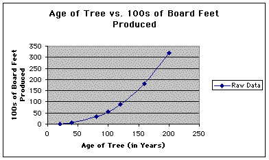
My next task was to find a function that best fit the given set of raw data. At first, judging by the shape of the graph, I thought that the function should be exponential. I quickly learned that exponential functions created more of a dramatic upward curve than I needed, so I moved on to a power function. After much guessing and testing, and while checking the residuals (explained below), I finally chose to use the function y = 0.00059x2.49.
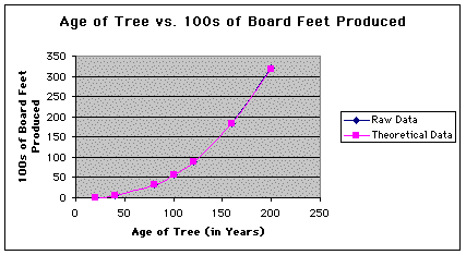
The following chart shows the given raw data set and the theoretical data set, which was found using the above function. Notice that the theoretical data is very close to the raw data.
|
|
|
|
|
|
|
|
| 20 | 1 | 1.02427530199162 |
| 40 | 6 | 5.75415279690848 |
| 80 | 33 | 32.3255616393263 |
| 100 | 56 | 56.3445625752648 |
| 120 | 88 | 88.7183210272092 |
| 160 | 182 | 181.597877598818 |
| 200 | 320 | 316.531328738118 |
The following figure is a graph of both the raw data set (in blue) and the theoretical data set (in pink). Note that the two curves seem to align so well that it is almost impossible to see the graph of the raw data set behind the graph of the theoretical data set.
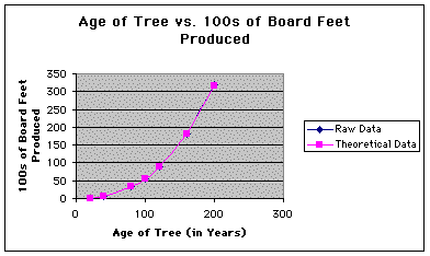
Now that I have decided on a function that I think best models the data, I can use it to predict missing data points. The spreadsheet performs this operation for me (see chart below).
|
|
|
|
|
|
|
|
| 20 | 1 | 1.02427530199162 |
| 40 | 6 | 5.75415279690848 |
| 60 | ??? | 15.7924178014801 |
| 80 | 33 | 32.3255616393263 |
| 100 | 56 | 56.3445625752648 |
| 120 | 88 | 88.7183210272092 |
| 140 | ??? | 130.229934006361 |
| 160 | 182 | 181.597877598818 |
| 180 | ??? | 243.489674632951 |
| 200 | 320 | 316.531328738118 |
I can predict that a 60-year-old tree produces approximately 1,600 board feet, a 140-year-old tree approximately 13,000 board feet, and a 180-year-old tree approximately 24,300 board feet.
Because the theoretical data set seems to match the raw data set so well, one can be led to believe that the function I chose could be the best function to use to model this data. Before that conclusion can be drawn, though, it is good to measure the error between the two sets of data.
The method I chose to use was to measure the residuals. First, I found the difference (called the residuals) between the theoretical data and the raw data. Since some of the residuals were positive and others were negative, it was not a good idea to average the residuals at this point. So, I squared the residuals in order to get a set of positive numbers, and then I averaged the squares.
Thes following chart shows all of the performed operations stated above.
|
|
|
|
|
|
|
|
|
|
|
|
| 20 | 1 | 1.02427530199162 | 0.0242753019916193 | 0.000589290286784317 |
| 40 | 6 | 5.75415279690848 | -0.245847203091518 | 0.0604408472679222 |
| 80 | 33 | 32.3255616393263 | -0.674438360673733 | 0.454867102348272 |
| 100 | 56 | 56.3445625752648 | 0.344562575264845 | 0.118723368273142 |
| 120 | 88 | 88.7183210272092 | 0.7183210272092 | 0.51598509813088 |
| 160 | 182 | 181.597877598818 | -0.402122401181515 | 0.161702425531987 |
| 200 | 320 | 316.531328738118 | -3.46867126188198 | 12.0316803230059 |
|
|
13.3439884548449 | |||
|
|
1.90628406497784 |
Note that the average of the squares of the residuals is approximately 1.9. The closer this value is to 0, the "better" the function that was chosen to model the data. It can be concluded that the function I used as a model is really good, but it is by no means to "best" function that exists.
Another way to analyze the residuals is to graph them, as shown below. Notice that most of the points seem to "bounce" between 0.7 and -0.7, which is fairly good. The last point, though, at a difference of -3.5, is an outlier of this trend. Again, it can be concluded that a better function can be found to model the data.
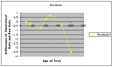
Since I concluded that a better function can be found to model the data than the one I had constructed, and because I had trouble finding a better one myself (using the guess-and-test method with the spreadsheet), I decided to compare my function with one generated by a graphics calculator.
For the same raw data set as previously used, a graphics calculator gave me the regression function y = 0.00058637x2.49260861. Obviously, this function is very close to the one I constructed, but it uses constants that have been taken out to more decimal places than the constants in my model. Because this new function is more accurate, it makes sense that it should be "better" than the one I chose to use.
Plugging this new function into the spreadsheet produces the following data set. Notice that the new theoretical data set is very similar to the theoretical data set that my function had produced.
|
|
|
|
|
|
|
|
| 20 | 1 | 1.02595972336347 |
| 40 | 6 | 5.77404641747198 |
| 80 | 33 | 32.4960242316547 |
| 100 | 56 | 56.6746651309192 |
| 120 | 88 | 89.2805420572102 |
| 160 | 182 | 182.885885307211 |
| 200 | 320 | 318.96198233571 |
A graph of this new theoretical data set (shown below) is almost exactly like the graph of the original theoretical data set that was produced by my function.
Even the predictions made using the new function (shown below) are not much different than those I made using my function!
|
|
|
|
|
|
|
|
| 20 | 1 | 1.02595972336347 |
| 40 | 6 | 5.77404641747198 |
| 60 | ??? | 15.8637866078776 |
| 80 | 33 | 32.4960242316547 |
| 100 | 56 | 56.6746651309192 |
| 120 | 88 | 89.2805420572102 |
| 140 | ??? | 131.107930616389 |
| 160 | 182 | 182.885885307211 |
| 180 | ??? | 245.29201274612 |
| 200 | 320 | 318.96198233571 |
One might conclude, then, that the accuracy of the constants in the model function is not so important. But the true story is revealed after analyzing the residuals that were produced by the new function. This information is shown in the chart below.
|
|
|
|
|
|
|
|
|
|
|
|
| 20 | 1 | 1.02595972336347 | 0.0259597233634659 | 0.000673907237107675 |
| 40 | 6 | 5.77404641747198 | -0.225953582528025 | 0.0510550214572488 |
| 80 | 33 | 32.4960242316547 | -0.50397576834532 | 0.253991575079256 |
| 100 | 56 | 56.6746651309192 | 0.674665130919223 | 0.455173038878252 |
| 120 | 88 | 89.2805420572102 | 1.28054205721016 | 1.63978796028402 |
| 160 | 182 | 182.885885307211 | 0.885885307210629 | 0.78479277753167 |
| 200 | 320 | 318.96198233571 | -1.03801766428995 | 1.07748067137797 |
|
|
4.26295495184552 | |||
|
|
0.60899356454936 |
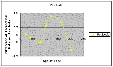
Note that the average of the squares of the residuals is now approximately 0.6, as opposed to 1.9 found before. 0.6 is closer to 0 than 1.9 is, so while the function produced by the graphics calculator is not perfect, it is definitely better than my function.
A graph of the residuals (below) supports the fact that the new function is better than the function I had constructed. Though the points still seem to "bounce around" a little, none of them are extreme outliers like the one produced using my function.
