

Objectives: To graph the sine and cosine functions; to identify the graphs of the sine and cosine functions.
"The sine and cosine functions are defined for all real numbers, and these functions have many real-world applications."
For example, "an oscilloscope is an electronic instrument used to display changing electrical signals. It displays electrical or sound waves as patterns on a flourescent screen. Many of the graphs shown on an oscilloscope are sine or cosine waves."
Resource: Hayden, Jerome D. and Hall, Bettye C. (1993). Trigonometry. Prentice Hall: Englewood Cliffs, New Jersey.
I. First, we must set up a table of the coordinates of some of the points that will satisfy the equation y = sinx.
1. Open an Excel spreadsheet. Label column A "x-coordinates" and column B "y-coordinates." Set both columns to round to 4 decimal places.
2. Fill in your x-coordinates in column A by ranging from 0p to 2p by increments of p/ 4. Remember, x represents an angular measure - we're using radians as our units.
3. Fill in your y-coordinates in column B by utilizing the equation, y = sinx.
What do you notice about the values in this column? Can you predict what the graph will look like?
II. Graphing in Geometer's Sketchpad.
1. Open GSP and choose a New Sketch. Go to the Graph Menu and select "Create Axes".
2. Go to the Graph Menu and select "Plot Points". Enter the values from your Excel spreadsheet. When finished, hit "Plot". You should have 9 points graphed.
3. Select the unit point on the x-axis and drag it to the right until the rightmost point of your graph is as far right as it can go without "falling" off the screen.
4. Select the 1st, 2nd, and 3rd points of your graph (from left to right) in that order. Go to the Construct Menu and select "Arc Through 3 Points". Then select the 3rd, 4th, and 5th points and do the same. Repeat the process for the 5th, 6th, and 7th and then the 7th, 8th, and 9th points.
You've just created the graph of a sine function!!
What is the domain of your graph? What is the range?
III. Extending the graph.
1. You have graphed the sine function from 0 to 2p. But a sine function is just like a line in that it goes on forever in two directions. So let's graph another part of the sine function by graphing the equation y = sinx from -2p to 0.
2. Follow parts I and II, but this time, let column A range from -2p to 0 by increments of p/ 4. Plot your points on the same graph as the one you just created.
What do you notice about the two parts of the sine function that you graphed?
IV. Check yourself.
Sketch (by hand!) what the graph of y = sinx will look like, given the following domain restrictions. Be careful about where the graph crosses the x-axis and where the graph reaches its maximum and minimum points.
a) 2p to 4p
b) -4p to 0
c) -3p to p
V. Save your GSP file. Call it sinwavesmu.gsp, where smu are your initials. Close the file.
I.
2. In cell A2, type in "0". In cell A3, type in "=A2+pi()/ 4". Drag to fill down to row 10.
3. In cell B2, type in "=sin(A2)". Drag to fill down to row 10.
Here is a sample table:
|
|
|
| 0 | 0 |
| 0.7854 | 0.7071 |
| 1.5710 | 1 |
| 2.3562 | 0.7071 |
| 3.1416 | 0 |
| 3.9270 | -0.7071 |
| 4.7124 | -1 |
| 5.4978 | -0.7071 |
| 6.2832 | 0 |
Note that the y-values seem to follow a pattern!!
II.
4. Here is a sample graph:
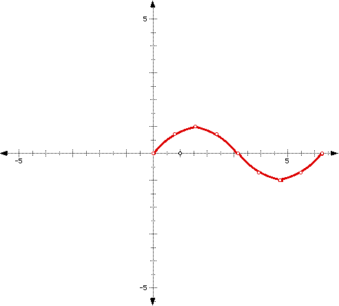
The domain of the graph is [0,2p] and the range is [-1,1].
III.
2. Here is a sample table:
|
|
|
| -6.2832 | 0 |
| -5.4978 | 0.7071 |
| -4.7124 | 1 |
| -3.9270 | 0.7071 |
| -3.1416 | 0 |
| -2.3562 | -0.7071 |
| -1.5710 | -1 |
| -0.7854 | -0.7071 |
| 6.2832 | 0 |
Here is a sample graph:
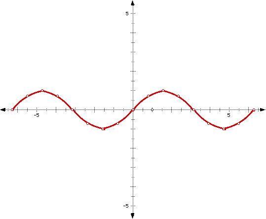
Note that the two "parts" of the graph are identical.
IV.
a)
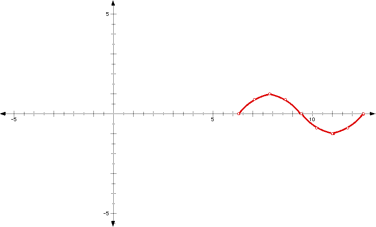
b)
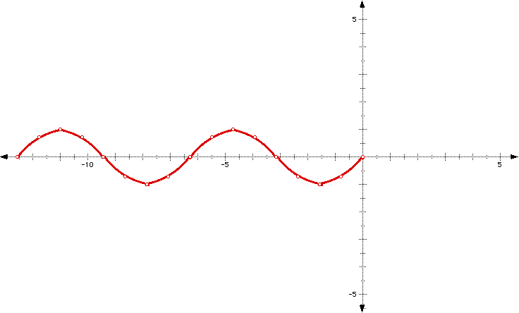
c)

I. First, we must set up a table of the coordinates of some of the points that will satisfy the equation y = sinx.
1. Open an Excel spreadsheet. Label column A "x-coordinates" and column B "y-coordinates." Set both columns to round to 4 decimal places.
2. Fill in your x-coordinates in column A by ranging from 0p to 2p by increments of p/ 4. Remember, x represents an angular measure - we're using radians as our units.
3. Fill in your y-coordinates in column B by utilizing the equation, y = cosx.
What do you notice about the values in this column? Can you predict what the graph will look like?
II. Graphing in Geometer's Sketchpad.
1. Open GSP and choose a New Sketch. Go to the Graph Menu and select "Create Axes".
2. Go to the Graph Menu and select "Plot Points". Enter the values from your Excel spreadsheet. When finished, hit "Plot". You should have 9 points graphed.
3. Select the unit point on the x-axis and drag it to the right until the rightmost point of your graph is as far right as it can go without "falling" off the screen.
4. Select the 1st, 2nd, and 3rd points of your graph (from left to right) in that order. Go to the Construct Menu and select "Arc Through 3 Points". Then select the 3rd, 4th, and 5th points and do the same. Repeat the process for the 5th, 6th, and 7th and then the 7th, 8th, and 9th points.
You've just created the graph of a cosine function!!
What is the domain of your graph? What is the range?
III. Extending the graph.
1. You have graphed the cosine function from 0 to 2p. But a cosine function is just like a line in that it goes on forever in two directions. So let's graph another part of the cosine function by graphing the equation y = cosx from -2p to 0.
2. Follow parts I and II, but this time, let column A range from -2p to 0 by increments of p/ 4. Plot your points on the same graph as the one you just created.
What do you notice about the two parts of the cosine function that you graphed?
IV. Check yourself.
Sketch (by hand!) what the graph of y = cosx will look like, given the following domain restrictions. Be careful about where the graph crosses the x-axis and where the graph reaches its maximum and minimum points.
a) 2p to 4p
b) -4p to 0
c) -3p to p
V. Save your GSP file. Call it coswavesmu.gsp, where smu are your initials. Close the file.
I.
2. In cell A2, type in "0". In cell A3, type in "=A2+pi()/ 4". Drag to fill down to row 10.
3. In cell B2, type in "=cos(A2)". Drag to fill down to row 10.
Here is a sample table:
|
|
|
| 0 | 1 |
| 0.7854 | 0.7071 |
| 1.5710 | 0 |
| 2.3562 | -0.7071 |
| 3.1416 | -1 |
| 3.9270 | -0.7071 |
| 4.7124 | 0 |
| 5.4978 | 0.7071 |
| 6.2832 | 1 |
Note that the y-values seem to follow a pattern!!
II.
4. Here is a sample graph:
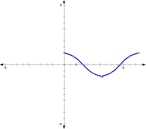
The domain of the graph is [0,2p] and the range is [-1,1].
III.
2. Here is a sample table:
|
|
|
| -6.2832 | 1 |
| -5.4978 | 0.7071 |
| -4.7124 | 0 |
| -3.9270 | -0.7071 |
| -3.1416 | -1 |
| -2.3562 | -0.7071 |
| -1.5710 | 0 |
| -0.7854 | 0.7071 |
| 6.2832 | 1 |
Here is a sample graph:
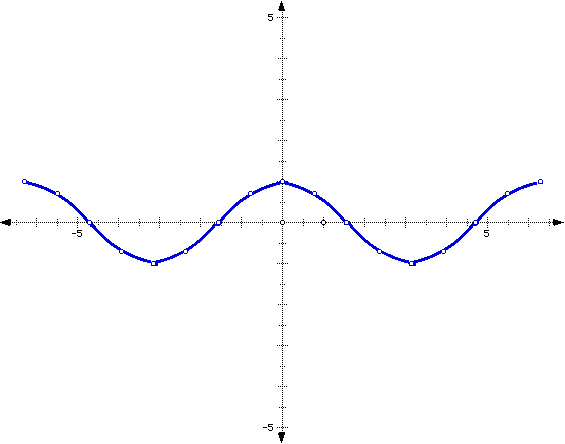
Note that the two parts of the graph are identical.
IV.
a)
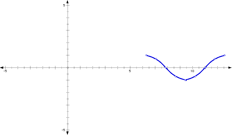
b)
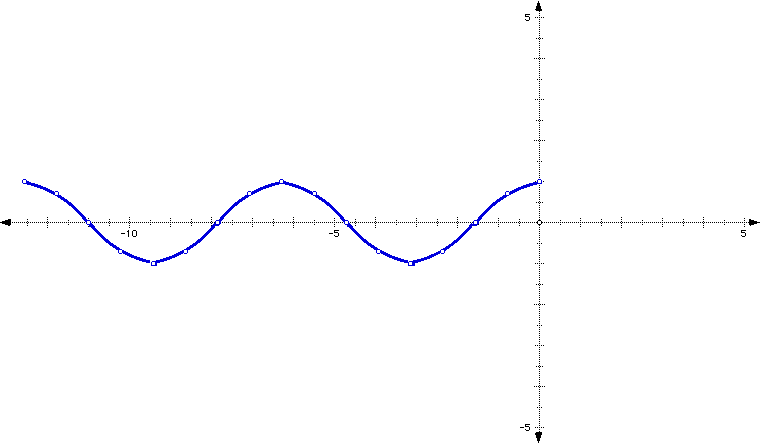
c)
1. Sketch the following functions over the given domain. Be careful about where the graph crosses the x-axis and where the graph reaches its maximum and minimum points.
a) y = cosx, [-2p, p]
b) y = sinx, [0, 3p]
c) y = sinx, [-p, p]
d) y = cosx, [p, 3p]
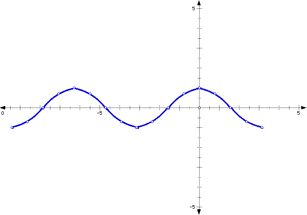
2. Give the function equation and the domain for the following graphs.
a)
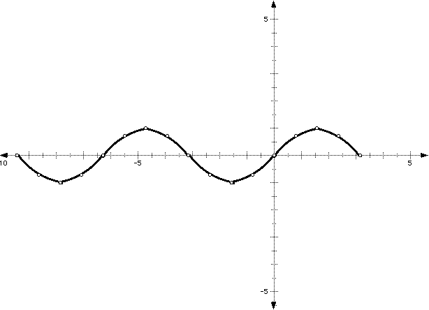
b)
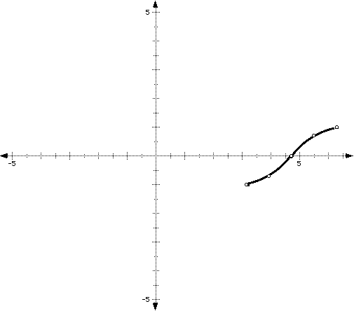
c)
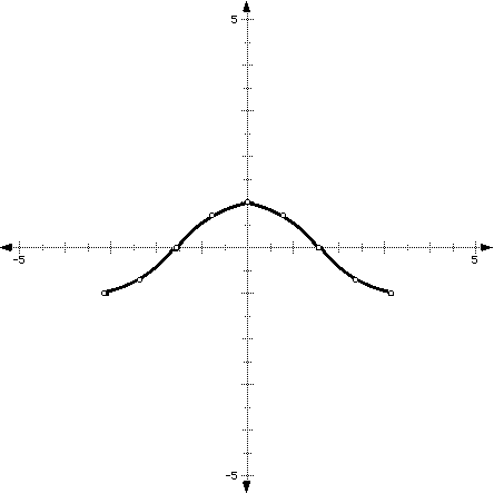
1.
a)
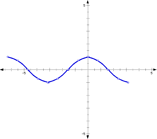
b)
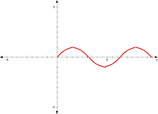
c)
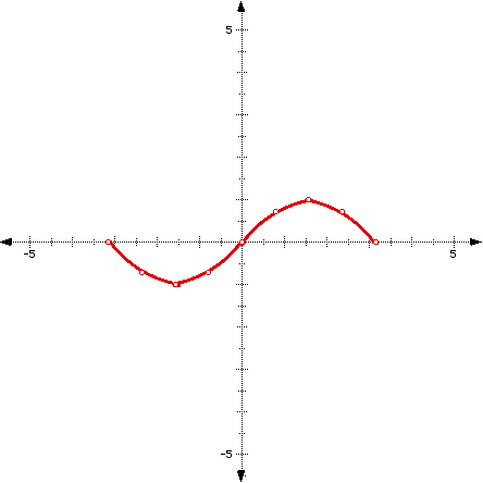
d)
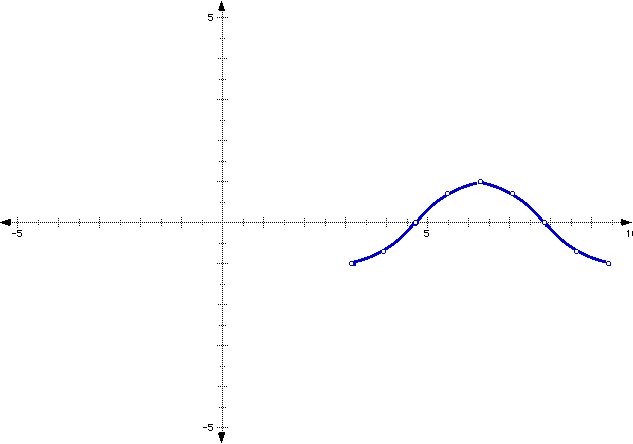
2.
a) y = sinx, [-3p, -p]
b) y = cosx, [p, 2p]
c) y = cosx, [-p, p]