
MAXIMIZING PROFIT
by Mary H. Bruce - EMAT 6690

Linear programming is typically taught in the secondary curriculum at the Algebra II level. I am always pleasantly surprised at the student response to this topic when I cover it with my classes. Students often struggle with inequalities and graphing. Thus, frequently I anticipate a negative reaction from the students when I show them the overlay of inequality graphs inherent to mathematical programming. Conversely, the students receive the topic well most likely due to the realistic, monetary nature of the problem. I believe both student interest and comprehension are heightened when a "real-world" value is made apparent by the teacher. In this essay I would like to incorporate technology to improve upon a student's understanding of maximizing profit and the balance between cost and revenue in the workplace.
An article in Mathematics Teacher, Vol. 92, No. 2 February 1999 titled "Promote Systems of Linear Inequalities with Real-World Problems" incorporates a hands-on approach by having students physically manufacture tables and chairs using Legos© building blocks. Students divide into corporate teams and see how many of each their group can make given the limited resources and then calculate the profit from each combination to find the one that generates the maximum profit.
I suggest one could alternatively employ a spreadsheet program to generate possible combinations, determine whether a combination is feasible and within the constraints as well as generate the profit from each to compare. Though both the hands-on and spreadsheet applications may be tedious and unrealistic in the large-scale sense, they initially enrich the student's understanding of the interplay between constraints, resources and process capability.
The problem as suggested in the article: A factory only manufactures tables and chairs. Each chair requires one large piece of stock and two small pieces of stock whereas a table requires two large and two small pieces. The profit on a chair and table are $15 and $20 respectively. The factory only has six large and eight small pieces of stock on hand.
Using Microsoft Excel, one can generate a spreadsheet outlining various combinations of products.
| # of chairs | # of tables | # of small stk | # of large stk | profit |
| 0 | 0 | 0 | 0 | 0 |
| 0 | 1 | 2 | 2 | 20 |
| 0 | 2 | 4 | 4 | 40 |
| 0 | 3 | 6 | 6 | 60 |
| 1 | 0 | 2 | 1 | 15 |
| 1 | 1 | 4 | 3 | 35 |
| 1 | 2 | 6 | 5 | 55 |
| 1 | 3 | 8 | 7 | 75 |
| 2 | 0 | 4 | 2 | 30 |
| 2 | 1 | 6 | 4 | 50 |
| 2 | 2 | 8 | 6 | 70 |
| 2 | 3 | 10 | 8 | 90 |
| 3 | 0 | 6 | 3 | 45 |
| 3 | 1 | 8 | 5 | 65 |
| 3 | 2 | 10 | 7 | 85 |
| 3 | 3 | 12 | 9 | 105 |
| 4 | 0 | 8 | 4 | 60 |
| 4 | 1 | 10 | 6 | 80 |
| 4 | 2 | 12 | 8 | 100 |
| 4 | 3 | 14 | 10 | 120 |
| 5 | 0 | 10 | 5 | 75 |
| 5 | 1 | 12 | 7 | 95 |
| 5 | 2 | 14 | 9 | 115 |
| 5 | 3 | 16 | 11 | 135 |
| 6 | 0 | 12 | 6 | 90 |
| 6 | 1 | 14 | 8 | 110 |
| 6 | 2 | 16 | 10 | 130 |
| 6 | 3 | 18 | 12 | 150 |
Notice that only the highlighted rows are within the capability of the company based on the limited resources of six large and eight small pieces of stock. One can easily find the combination that fully utilizes its resources to the greatest potential - when the company makes 2 chairs and 2 tables, the resources are fully utilized and the profit is maximized at $70. The other highlighted feasible combinations only partially utilize the resources as evident from the spreadsheet. Students quickly realize that perhaps their preliminary notion of making as many tables as they can since it has the highest profit margin is not necessarily the best use of the company's resources.
Using Nucalc, one can easily generate a graph of the feasible region given the company constraints and resources. Only the first quadrant would apply given the realistic nature of the problem. In this graph, the x coordinate represents the number of chairs manufactured and the y coordinate represents the number of tables. The following inequalities apply: x >= 0, y >= 0, x + 2y <= 6 (lg stock constraint), 2x + 2y <= 8 (sm stock constraint):

Notice the dark gray enclosed region contains the feasible combinations of the company. Due to the integral nature of the chairs and tables, only points where gridlines cross within the feasible region are actual possibilities. One can count 13 such possibilities within the region thus corresponding with the 13 highlighted possibilities in the excel spreadsheet.
Next one can enter the profit equations. Since the chairs generate a profit of $15 and the tables generate a profit of $20, the profit equation would be of the form 15x + 20y = Total Profit. Looking at the excel spreadsheet one notices the possible profit values of 0, 15, 20, 30, 35, 40, 45, 50, 55, 60, 65 and the maximum 70. Graphing the linear profit equations atop the feasible region, one can easily match the chair/table combinations with their appropriate profit value by looking where the profit lines pass through grid intersection points within the feasible region. If students plot the individual profit equations one at a time they will notice that the larger the profit value, the higher the line falls.
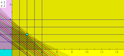
One notices the highest of the parallel profit equations (thus highest profit) passes through the point (2,2) of the feasible region thus acknowledging the 2 chair, 2 table combination previously determined.
Suppose the profit margins were different though available resources the same: Let a chair have a $20 profit margin and a table have a $15 profit margin. Using an excel spreadsheet makes it easy to rerun the numbers with a different profit calculation:
| # of chairs | # of tables | # of small stk | # of large stk | profit |
| 0 | 0 | 0 | 0 | 0 |
| 0 | 1 | 2 | 2 | 15 |
| 0 | 2 | 4 | 4 | 30 |
| 0 | 3 | 6 | 6 | 45 |
| 1 | 0 | 2 | 1 | 20 |
| 1 | 1 | 4 | 3 | 35 |
| 1 | 2 | 6 | 5 | 50 |
| 1 | 3 | 8 | 7 | 65 |
| 2 | 0 | 4 | 2 | 40 |
| 2 | 1 | 6 | 4 | 55 |
| 2 | 2 | 8 | 6 | 70 |
| 2 | 3 | 10 | 8 | 85 |
| 3 | 0 | 6 | 3 | 60 |
| 3 | 1 | 8 | 5 | 75 |
| 3 | 2 | 10 | 7 | 90 |
| 3 | 3 | 12 | 9 | 105 |
| 4 | 0 | 8 | 4 | 80 |
| 4 | 1 | 10 | 6 | 95 |
| 4 | 2 | 12 | 8 | 110 |
| 4 | 3 | 14 | 10 | 125 |
| 5 | 0 | 10 | 5 | 100 |
| 5 | 1 | 12 | 7 | 115 |
| 5 | 2 | 14 | 9 | 130 |
| 5 | 3 | 16 | 11 | 145 |
| 6 | 0 | 12 | 6 | 120 |
| 6 | 1 | 14 | 8 | 135 |
| 6 | 2 | 16 | 10 | 150 |
| 6 | 3 | 18 | 12 | 165 |
Notice that although the company resources remain the same, the change in profit margins affect the maximum combination. The green highlighted row shows us the new 4-chair, 0-table combination for a maximum profit of $80. Can the students intuitively understand this change from a business perspective? The chairs require fewer resources but yet have a higher profit than the tables. Of course a company would want to maximize production of such a product. This questioning can even unexpectedly then lead into discussion of excess supply versus diminishing demand.
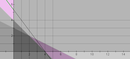
Using Nucalc and plotting the profit equation 20x + 15y = 80, one notices the profit line passes through the grid intersection at (4,0):
Finally, suppose a chair had a $15 profit margin and a table had a $40 profit margin:
| # of chairs | # of tables | # of small stk | # of large stk | profit |
| 0 | 0 | 0 | 0 | 0 |
| 0 | 1 | 2 | 2 | 40 |
| 0 | 2 | 4 | 4 | 80 |
| 0 | 3 | 6 | 6 | 120 |
| 1 | 0 | 2 | 1 | 15 |
| 1 | 1 | 4 | 3 | 55 |
| 1 | 2 | 6 | 5 | 95 |
| 1 | 3 | 8 | 7 | 135 |
| 2 | 0 | 4 | 2 | 30 |
| 2 | 1 | 6 | 4 | 70 |
| 2 | 2 | 8 | 6 | 110 |
| 2 | 3 | 10 | 8 | 150 |
| 3 | 0 | 6 | 3 | 45 |
| 3 | 1 | 8 | 5 | 85 |
| 3 | 2 | 10 | 7 | 125 |
| 3 | 3 | 12 | 9 | 165 |
| 4 | 0 | 8 | 4 | 60 |
| 4 | 1 | 10 | 6 | 100 |
| 4 | 2 | 12 | 8 | 140 |
| 4 | 3 | 14 | 10 | 180 |
| 5 | 0 | 10 | 5 | 75 |
| 5 | 1 | 12 | 7 | 115 |
| 5 | 2 | 14 | 9 | 155 |
| 5 | 3 | 16 | 11 | 195 |
| 6 | 0 | 12 | 6 | 90 |
| 6 | 1 | 14 | 8 | 130 |
| 6 | 2 | 16 | 10 | 170 |
| 6 | 3 | 18 | 12 | 210 |
One notices the highlighted combination of 0-chairs, 3-tables for a maximum profit of $120. The Nucalc graph shows the profit line passing through the point (0,3):
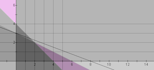
Looking at the past few examples and the feasible polygon and polygonal interior of values, perhaps the students themselves will notice the maximum profit seems to always occur at the corner points. Through technology, students gain a richer understanding of the corner principle of linear programming, and acceptance is more assured and definite.
Does cost always have to be linear? Perhaps class discussion reminds students of maximum/minimum problems with quadratic functions. If a company is not utilizing its building and equipment fully and not producing many items, the cost per item produced may be high. As the company produces more and more items with the same given space and equipment, the cost per item will decline until possibly the rising production of items causes the company to outgrow the building and equipment thus forcing the company to expand. As the company expands, the cost per item will then increase again. Students can visualize a possible quadratic cost function.
Suppose the Puppy Dog Food Company sells a sack of dog food for $2. The cost of manufacturing a sack of food is represented by the function C(x) = 0.25x² - 5x + 27. Determine the profit function, the number of sacks of food that maximizes profit and the associated profit.
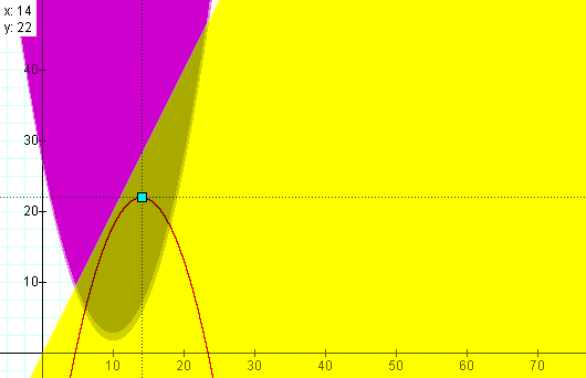
Looking at the graph, one notices the shaded region represents the area where the linear revenue function exceeds the parabolic cost function and, thus, profit is generated. The equation for the profit function (the difference of the revenue function and the cost function) is graphed by the red parabola, and one can see the maximum profit of $22 occurs at 14 sacks of food. By using graphs to show the separate functions, students make sense of break-even production, profit and loss.
RETURN to Mary's Class Page