

It has now become a rather standard exercise, with availble
technology, to construct graphs to solve the equation
and to overlay several graphs of
for different values of a, b, or c as the other two are held constant.
From these graphs, roots of
can be estimated or actually found and other patterns or methods for solving such roots may be boldly explored.
For example, if we set
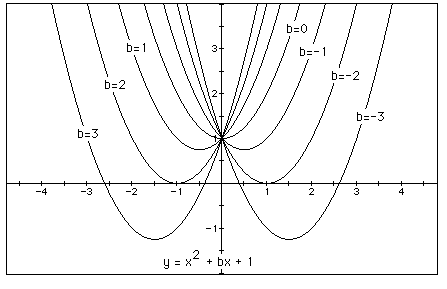
for b = -3, -2, -1, 0, 1, 2, 3, and overlay the graphs, the
following picture is obtained.
Click here for a live demonstration of how the above parabola changes as b = (-10,10).
It becomes obvious which functions have real roots and which
ones do not, but furthermore we can discuss the "movement"
of a parabola as b is changed. The parabola always passes through
the same point on the y-axis ( the point (0,1) with this equation).
For b < -2 the parabola will intersect the x-axis in two points
with positive x values (i.e. the original equation will have two
real roots, both positive). For b = -2, the parabola is tangent
to the x-axis and so the original equation has one real and positive
root at the point of tangency. For -2 < b < 2, the parabola
does not intersect the x-axis -- the original equation has no
real roots. Similarly for b = 2 the parabola is tangent to the
x-axis (one real negative root) and for b > 2, the parabola
intersets the x-axis twice to show two negative real roots for
each b.
After briefly analyzing the locus of the vertices of the set
of parabolas graphed from
we have numerous conceptual and applied options when we introduce
a new function to the mix.
Consider
being introduced to the family of curves above.
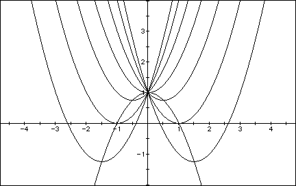
Click here and view the interaction as b is allowed to vary.
Consider again the equation
Now graph this relation in the xb plane. We get the following
graph.
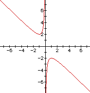
If we take any particular value of b, say b = 3, and overlay
this equation on the graph we add a line parallel to the x-axis.
If it intersects the curve in the xb plane the intersection points
correspond to the roots of the original equation for that value
of b. We have the following graph.
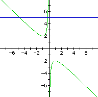
For each value of b we select, we get a horizontal line. Click here to see an active demonstration of this.
What do you notice happens to the line with certain values of b?
It is clear on a single graph that we get two negative real
roots of the original equation when b > 2, one negative real
root when b = 2, no real roots for -2 < b < 2, One positive
real root when b = -2, and two positive real roots when b <
-2.
Consider the case when c = - 1 rather than + 1.
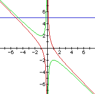
One may view or create similar graphs in graphing calculator 3.1 by these functions of x and y
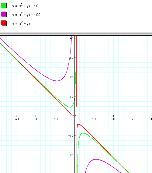
In the following example the equation
is considered. If the equation is graphed in the xc plane,
it is easy to see that the curve will be a parabola. For each
value of c considered, its graph will be a line crossing the parabola
in 0, 1, or 2 points -- the intersections being at the roots of
the orignal equation at that value of c. In the graph, the graph
of c = 1 is shown. The equation
will have two negative roots -- approximately -0.2 and -4.8.
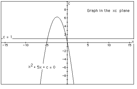
There is one value of c where the equation will have only 1 real root -- at c = 6.25. For c > 6.25 the equation will have no real roots and for c < 6.25 the equation will have two roots, both negative for 0 < c < 6.25, one negative and one 0 when c = 0 and one negative and one positive when c < 0.
In closing, these explorations can be widely adaptable to different levels of students and grade levels. This may be a good opportunity to introduce asymptotes and limits at a conceptual level for Algebra 2 and Pre Calculus students.
Return to Jeff Daniel's web page