
Janet Kaplan
POLAR EQUATIONS
_____________________________________________________________________________________________________________
We are most familiar with functions as they
appear when graphed on the rectangular coordinate plane. But often it is easier
to work with the polar coordinate system
of representation, particularly when describing motion using a function of one
variable. The polar coordinate system
facilitates the study of circular motion.
It is extremely useful when describing the motion of electrons around
the nucleus of an atom or the circular paths of orbiting spacecraft.
In this investigation we will look closely
at several well-known polar equations and determine what gives them their
characteristic shape.
Before
we begin our exploration, however, it may be useful to review how polar
equations are graphed. CLICK HERE
for a review of polar coordinates from Math Forum.
Let’s take a look, first of all, at the
function r = a + b cos (kt).
where a,
b and k are positive integers, b is the coefficient of the
trigonometric function, t is the angle measurement, and k
is its coefficient.
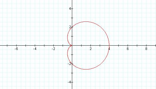
Polar equations of this form are known as limacons (for the French word for
snail). When a = b, we get a special case of the limacon. The resulting graph
is called a cardioid because of its
heart like shape.
r = 2 + 2 cos (t)
But if we vary the values of a and b, the
respective limacons take on different looks, as in the graph below.
r = 1 + 2 cos (t) r = 2 + 2 cos (t) r = 3 + 2 cos (t) r =
5 + 2 cos (t)
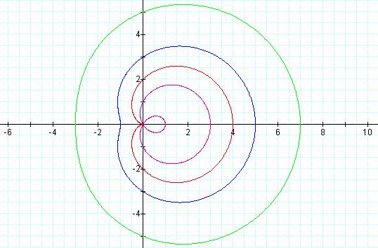
As you might expect, there are reasons for
the changing shape. Limacons can be
characterized according to the relative sizes of a and b.
r = 1 + 2 cos (t) is an example in which a < b
r = 2 + 2 cos (t) is the cardioid, in which a = b
r = 3 + 2 cos (t) is a case in which b < a < 2b and
r = 5 + 2 cos (t) is a case in which a >= 2b
_____________________________________________________________________________________________________________
Now let’s look at a polar equation which is
seemingly more basic, but has some beautiful designs in store for us.
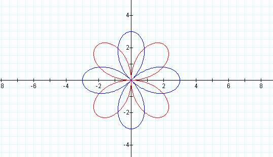
r = b cos (kt)
Getting rid of the additional term, but varying
the value of the coefficient k, we
come across the lovely n-leaf rose.
r = 3 cos (1t) r = 3 cos (3t)
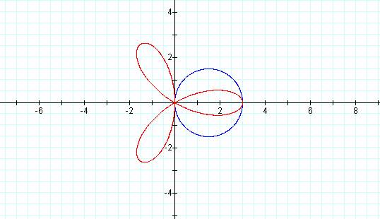
r = 3 cos (2t) r = 3 cos (4t)
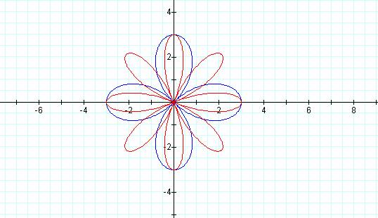
Notice how the number of petals corresponds to
the value of k. When k is 1, there’s just the lone petal hanging to the right
of the y-axis stalk. When k = 3, we get 3 petals. But when k = 2 or 4, we get 4
and 8 petals, respectively. The pattern
seems to be that when k is odd, the number of petals is equal to k. But when k is even, the number of petals is
equal to 2k. Now why would this be?
Well in fact, it’s really just an illusion.
When k is odd, the points of each petal are traced twice as t ranges from 0 to
2Pi. If k is even, the trace of each petal
is drawn once, changing its orientation slightly around the origin, as t ranges
from 0 to 2Pi.
_____________________________________________________________________________________________________________
What is the significance of the value of b? As
the graph below indicates, the value of b determines the length of the leaf.
r = 1 cos (5t) r = 2 cos (5t) r = 3 cos (5t)
_____________________________________________________________________________________________________________
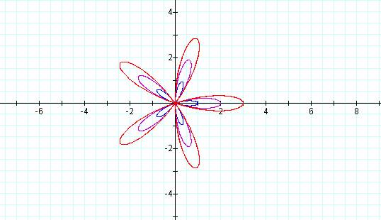
How does cos (t) compare with sin (t)?
r = 3 cos (2t) r = 3 sin (2t)
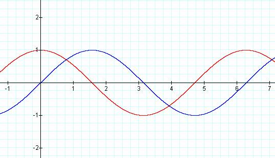
Notice how the sine function is rotated 45
degrees from the cosine function. Just like in the rectangular coordinate
system shown below, the two trigonometric functions are “out of phase” from
each other by 45 degrees or (pi / 4).
_____________________________________________________________________________________________________________