Cooling water
Write-up by
Blair T. Dietrich
EMAT 6680
Assignment #12 problem #8
This exploration involves modeling data that was collected by heating a cup of water and then measuring the temperature of the water each minute for thirty minutes. A Texas Instruments CBL2 with temperature probe was used to collect the temperature data. According to the temperature probe the room temperature at the time of the experiment was 78.1 degrees Fahrenheit.
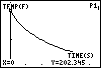
The initial temperature of the water was measured to be 202.345˚F. The water was allowed to cool and after thirty minutes the water temperature was measured to be 120.729˚F. A screenshot of a graphical representation of the collected data is shown below:

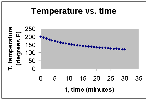
Using Microsoft Excel, a scatter plot of the data was created:

According to Newton's Law of Cooling, "the temperature
of a heated object decreases exponentially over time toward the temperature of
the surrounding medium." That is,
the temperature T of a heated object at a given time t can be
modeled by the function ![]() , where R is the constant temperature of the
surrounding medium,
, where R is the constant temperature of the
surrounding medium, ![]() is the initial
temperature of the heated object, and k is a negative constant (page
478, College Algebra, 5th edition by Sullivan).
is the initial
temperature of the heated object, and k is a negative constant (page
478, College Algebra, 5th edition by Sullivan).
In this case, R = 78.1˚F and ![]() = 202.345˚F, so
the model should approximately be of the form
= 202.345˚F, so
the model should approximately be of the form

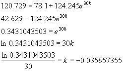
In order to find the best approximation for k (and
thus the best model using these values of R and ![]() ), I chose to substitute my last data point (30, 120.729)
into the preceding equation and solve for k as follows:
), I chose to substitute my last data point (30, 120.729)
into the preceding equation and solve for k as follows:

Thus, a reasonable model should be ![]() .
.
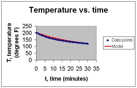
This model is shown below in red, superimposed on the scatter plot of the data.

The model that has been obtained can now be used to predict T for future values of t:
For t = 45, ![]()
![]()
For t = 60, ![]()
For t = 300, ![]()
Predictions such as these that are outside the range of the known data are said to be extrapolations based on the model. As long as we expect the data trend to continue in the same pattern that we have observed, we should feel confident that our predictions are reasonable. The last extrapolation indicates that, had the water been allowed to cool for 300 minutes (5 hours), the water temperature would have approximately been at the room temperature.
Although we expect there to be an exact relationship between the temperature of the water and the elapsed time, we realize that random error is involved with each individual data point that we have obtained. Thus, our model necessarily includes a random error component.ε that we expect to cancel out overall (i.e. the expected value of ε will be zero) so we do not expect our model to fit the data exactly (as can be seen in the graph above).
One measure of error is the Mean Square Error (MSE). This is found by finding the residuals (observed values – predicted values). The sum of the squares of the residuals is then found and divided by the number of data points. The smaller the value of MSE, the "better" the model. For this model, the MSE is 43.43153.
For comparison, I used a TI-83+ calculator to generate the
exponential equation of best fit for this data. The regression process finds the exponential equation that will
yield the least error of estimate. The
model that I generated for this data was ![]() . For this model, the
MSE is 10.32777. The regression model
is, overall, a better model. However,
its initial value of 190.69˚F is quite different than the observed initial
water temperature.
. For this model, the
MSE is 10.32777. The regression model
is, overall, a better model. However,
its initial value of 190.69˚F is quite different than the observed initial
water temperature.