This assignment is concerned with demonstrating the properties and behavior of quadratic functions. I will make graphs of quadratic functions varying the coefficients in a systematic manner and explain the results as though the presentation is for a College Algebra Class.

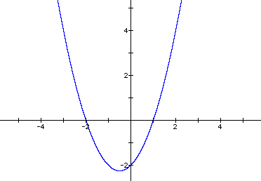
The graph of this equation has a y-intercept of -2 as expected and x intercepts of -2 and 1. The vertex of this graph is at (-0.5, -2.25). Now see what happens to the graph when c is changed to -1.5.

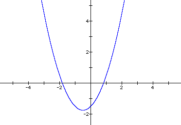
The whole graph has moved upwards 0.5 units. We call this a vertical shift. The y intercept is now -1.5 and the vertex is now (-0.5, -1.75). Does this always happen when we increase c by some amount? We increased c by 0.5 from the previous graph to get the current graph. Suppose we now increase c by 1 just to test our question. The graph with c = -0.5 appears below.

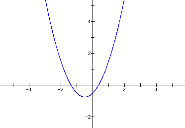
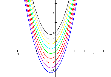
Yes, the whole graph shifted upwards by one unit. The y-intercept is now -0.5 and the vertex is now (-0.5, -0.75). Notice that one odd thing is happening, or is it odd?. The y-coordinate of the vertex is increasing at the same rate as c, but the x-coordinate of the vertex is remaining constant at -0.5. Remember from the lecture that the x-coordinate of the vertex is always -b/2a. Since we are not varying a or b, this is not such a strange behavior. The graph below shows the effect of varying c from -2 to 2 and also shows the locus of the vertex as the vertical line x=-0.5.

Now we will look at equations of the form . We will begin with the graph of the equation .

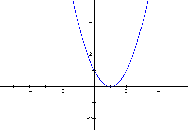
The shape of the graph has not changed, but then we didn't expect it to. All quadratic functions graph as parabolas. The y=intercept is (0, 1) as expected. (Remember, to get the y-intercept we set x to zero and solve for y.) The vertex is at (1, 0). The vertex coincides with the x-intercept, of which there is only one. If you set y to zero and solve the resulting quadratic equation for x, the solutions you get will coincide with the x-intercepts. You can use this fact to solve quadratic equations graphically if you wish. First graph the equation. Then notice the locations of the x-intercepts. These are the solutions of the quadratic equation. However, we want to vary b and see what happens to the graph. Let's let b = -1.5.

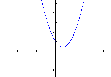
This is quite a bit different from the effect we got by changing c from -2 to -1.5. This time the graph has moved upwards some amount and to the left by some smaller amount while the y-intercept has remained fixed at y=1. (We sort of expected the y-intercept to remain at y=1 didn't we? Why?) Let's find the coordinates of the vertex. Using the method we learned in the lecture, the vertex is now at (0.75, 0.5625). So the vertex moved up 0.5625 units and to the left 0.25 units.Will this happen every time we increase b by 0.5? Let's see the graph for b=-1.

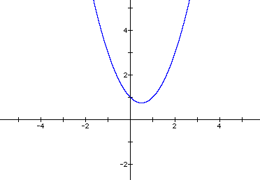
Well, the graph did move upward and to the left. But, did it move by the same amount? If we find the vertex of this graph we find it is (0.5, 0.75). The graph did move to the left by the same amount (0.25), but not as far upward. The graph only moved upward 0.1875. How is 0.1875 related to 0.5625? We will explore that question a little later. First, let's look at the family of graphs that we get by varying b from -2 to 2 in steps of 0.5. I will also include the graph of the locus of the vertices on this graph.

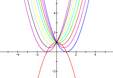
Aha! The vetices move up and to the left for -2 < b < 0 and down and to the left for 0 < b < 2. As a matter of fact, the locus of the vertices seems to be a parabola. Is that true? Yes! The explaination appears below.

Can we determine the equation that coincides with the locus of the vetices? Try this:

In fact, that is exactly the equation of the red parabola above.

Finally, we will look at the graphs of equations of the form . We will begin with the graph of the equation .

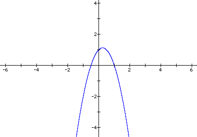
This graph has x-intercepts at x= -1/2 and x = 1, a y-intercept at y = 1, and the vertex at (0.25, 1.125). Let us see what happens if we let a = -1.5. See below.

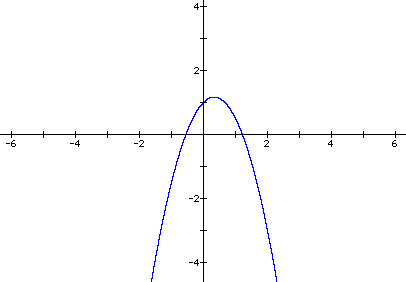
There doesn't seem to have been much change here. Let's see just how much. It is obvious that the roots have changed because the x-intercepts are different. Let's take a look at the movement of the vertex. The new vertex is (0.333, 1.167). So the vertex moved to the right by .083 and upwards by 0.042. Let's increase a by 0.5 again and see if we get the same results. The graph below is for a = -1.

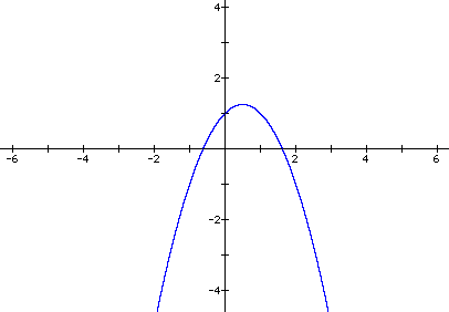
Again, there doesn't seem to be much change. However, the new vertex is at (0.5, 1.25), a movement of 0.167 to the right and .083 upward. Let's check the line through the last two vertices and see if the first vertex is on the line. Then we can see if we can predict the coordinates of the next vertex when a = -0.5. From our previous study of straight lines we know that if we are given the coordinates of two points on a line we can determine the equation of that line by determining the slope of the line and then using the point-slope form for the equation of a line.

Substituting the x-coordinate of the first vertex into this equation we get y= 1.125 as expected. So we conclude that the coordinates will have a locus along the line y = 0.5x +1. Let's check this out. Let a = 0.5 (a = 0) is trivially the line y=x+1.).

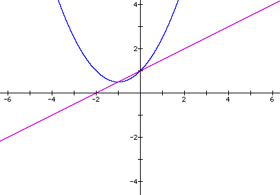
I have added the line y = 0.5 x + 1 to see if our assumption was correct. Notice that now the parabola opens upward instead of downward. However, the vertex is on the line y = 0.5x +1 as we hoped. Evidently the sign of a determines the orientation, upward or downward of the parabola. You can experiment for yourselves to see that this is true. Below is the graph of our equation for values of a from -2 to 2 in steps of 0.5 along with the line y = 0.5 x+1.

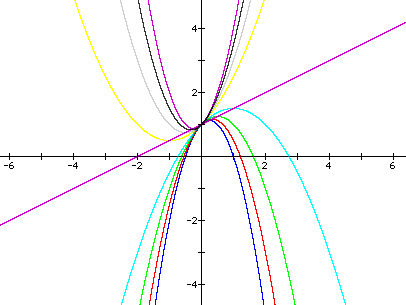
All of the graphs have a y-intercept at y = 1 and all of the vertices are on the line y = 0.5x + 1.

We have shown how the graphs of parabolas react to changes in the coefficients when the coefficients are varied singly. For further exploration, you might want to investigate how the graphs respone to a systematic variation of two of the coefficients at a time.

Return