
The idea of this project is to take observed data and generate a function that best represents that data. In this project their were three explorations that were used in the generation of the function that fit the observed data best.
1. Take a cup of hot water and measure its initial temperature(time=0). Then, record temperature readings each minute for 30 minutes. Make sure to make note of the room temperature.
2. Enter the data into a spreadsheet and plot the observed data versus time. Now generate a function that models the data that you just compiled.
3. To aid in the determination of the function that best represents your data, calculate a measure of error between the observed data and your model. One such error measure is the average of the square of the differences at each time. This is calculated by taking the square of the differences at each time, summing them up and dividing by the number of data points. The number that results lets you know how well your model fits the observed data. When generating a function to model the data, if the average of the square of the differences increases, this tells you that the change you just made to your model made your model a worse representation of the observed data than you had previously. Likewise, if the average of the square of the differences decreases, this tells you that the change you just made to your model made your model a better representation of the observed data than you had previously.
Below are the temperature readings for the first thirty minutes that the water was cooling. I started taking measurements when the water reached its boiling point(212 degrees Fahrenheit).
| Time(min.) | Time(min.) | |||
From this data, I plotted temperature versus time to get an idea of what the function that I would need to model this data would look like. Figure 1 below displays this graph.

As one would have expected, the curve of the observed data is a continous decreasing function. This curve looks like some type of a decreasing exponential function. The exponential function modeling the observed data will look similar to the following:
Since the temperature of the water can never be less than room temperature, under normal conditions, the room temperature observed in this experiment(which was observed to be 72 degrees fahrenheit) must be a constant(C) in the function that models the observed data because for any time after the time when the water has cooled to 72 degrees the observed temperature of the water should remain at 72 degrees. Also since the slope of the tangent lines to the curve in Figure 1 are all negative, the value of x in the exponential function modeling the data must also be negative. The A in the equation above is also a constant. At the initial time(time=0), the temperature was 212 degrees, therefore knowing that the room temperature was 72 degrees the equation above for x=0 must equal 212. Thus A must equal 140. The t is in the equation because we need to be able to find temperatures at different times. Now the above equation looks like the following:
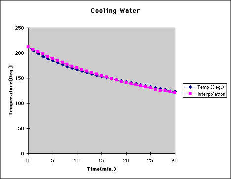
Now using a spreadsheet program(or some other program), this function can be combined with the observed data to find a value for x that makes the function model the observed data as best as possible. One can use the square of the differences discussed above to get a value for x that allows the function to best represent the curve of the observed data. After trying many different values for x, the value x=0.035302 gave a very good model of the observed data. Figure 2 illustrates how well the function above modeled the observed data.

Now that a function is defined that models the observed data fairly well, this function can be used to extrapolate what the temperature of the water will be after time=30 minutes. For example, the temperature after
Time(min.) Temp.(F) 45 100.59 60 88.84 300 72.01
The data displayed in this experiment is dependent on many factors.
These are only a few of the factors that the data in this experiment and other experiments like this one are dependent on. Some of these factors can be made minimal with great attention to detail and other precautions.