

This investigation focuses on polar equations and their graphs. The polar coordinate system is related to the Cartesian coordinate system generally taught in the school systems. Students can be taught how to transform many equations from one system to the other.
The polar coordinate system resembles that of a circular graph. Its origin is called the pole. It is a fixed point that has a ray extending from it, also fixed. The ray is known as the intial ray.
Each point can be defined as a polar coordinate using two directives. The first is r, the length of the ray from the pole. The second directive is the angle from the inital ray. Generally the angle is written as theta. In this investigation, we will refer to it as simply t.
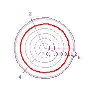
The image above is the picture of the polar equation r = 1. As was described in the beginning paragraphs, the pole is the origin of the polar coordinate system. This has the value of 0. It correlates with the origin on a Cartesian coordinate system. The initial ray, in the image, corresponds to the x-axis on a Cartesian coordinate system.
Remember that r represents the length of the inital ray. Therefore it is not surprising that our initial ray (from the origin) has the length of 1. The circular image is created by the fact that our equation does not give us a restriction on the size of theta, the angle. Thus, we need to plot all of the points where the length of the ray is 1. This becomes a circle.
This graph may be a nice equation to illustrate the relationship between the polar coordinate system and the Cartesian coordinate system.
Polar coordinates can be defined using the typical Cartesian coordinate system

If we apply the general Cartesian coordinate system for a circle, we would have
In this particular case we have our radius equal to 1, therefore our equation would be
We substitute our equivalent polar expressions into this equation and get
Factoring leaves us with
Substituting our trigonometric identity gives
Therefore
Our first exploration will be when a = b, namely a = b = 1. I will vary k using values from 0 to 10. The first graph is r = 1 + 1 cos (0t). Before graphing the equation, let's determine some of the points that will be plotted. When we substitute 0 in for theta, the value of cos(0) is 1. Our equation then becomes r = 1 + 1 or r = 2. This is almost identical to the graph we explored previously, except that the length of the ray will be 2.
Let's begin our graphing with k = 1. The equation then becomes r = 1 + 1 cos(1t).
The graph is as follows:
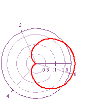
The shape is called a cardoid. It is created by plotting all of the points that satisfy the above equation when the angle theta is increased from 0 to 2pi. The indentation on the left is created because the values of cos(t). For example the the cardoid intersects the circle of radius 1 at the value of pi/2. This is because the cos(pi/2) is zero and when we substitute it into our equation r = 1 + 1 cos(t) r = 1 + 0. Our equation plots the point at (1, pi/2) (r,theta). The 'dimple' on the left is created because the value of cos(pi) equals -1. When we place that into our equation, we find that r = 1 + 1cos(pi) becomes r = 1 + (-1) at pi. The point is (0, pi).
The next image is graph of the equation r = 1 + 1 cos(2t). This means that every value of theta is doubled before it is evaluated with cosine. (0 pi continues to be 0 pi; pi/2 becomes pi; pi becomes 2pi; 3pi/2 becomes 3pi; 2pi becomes 4pi). The image shows the effect doubling theta will have on the graph.
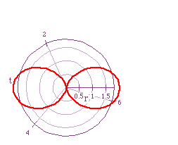
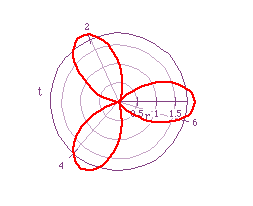
Let's look at r = 1 + 1 cos (3t)
And r = 1 + 1 cos (10t)
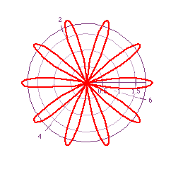
This shape is generally known as the n-leaf rose. Notice that the coefficient before theta determines the number of 'petals' on the picture. We also notice that our petals reach out to the length of the ray when theta is 0. This makes the length of the ray to be 2.
We will begin by substituting 0 in for theta. Our equation will become
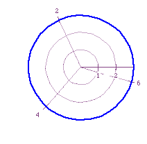
We should notice in this graph that our points have been plotted as the ray = 3 is rotated for the values of theta 0 to 2pi. This graph does not look that much different than our previous graph. Let's continue to look at another graph and compare it.
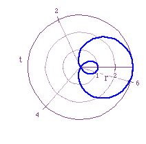
Our equation now creates a loop inside the cardoid. This shape is known as a limacon. This image is produced when values for r are negative.
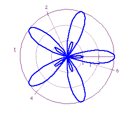
As we continue to investigate other equations and their graphs look for a pattern. The next image is the graph of r = 1 + 2 cos (3t).
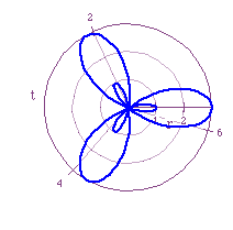
The figure now becomes the n-leaf rose with an imbedded n-leaf rose. In the imbedded figure the petals reach a length of 1.
The figure r = 1 + 2 cos (10t) holds this pattern.
Let's constrast the previous graphs with new graphs where a > b.
We will, once again, begin with the substitution of zero as theta. Our equation becomes r = 2 + 1 cos (0t). Do we expect to see a graph that is different than the previous graphs with zero as theta? We would hope not.
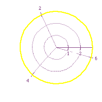
Our graph looks as we expected it to. The previous arguments hold for this equation and figure.
Let's continue to explore and graph r = 2 + 1 cos (1t).
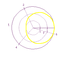
Our graph, already, takes on a different look. The dimple and loop that we had seen in the previous graphs (when k = 1) are not as prominent in this graph. To explain this graph, we must look at what is happening when theta = pi. The value of cos(pi) is -1. When we evaluate this in our equation (r = 1 + (-1)), we see that our point will be at (1, pi). To produce the loop, some values of r must be negative. Therefore, the graph is being affected by changing the beginning number to 2.
The following image is the graph r = 2 + 1 cos (3t)
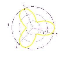
This graph, again, is different than the graphs that we have seen before. The n-leaf pattern is still present, yet the indentations are not touching each other. The points that help to create these indentations never hit a point that is lower than 1 because of the equation that we have set up.
Let's look at r = 2 + cos (5t)
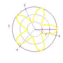
The pattern holds in this image as well. As we can see, our image does not have any points that have r < 1. This can lead to a nice discussion about the effects of the values of cos (t) on the graph.
More specifically, we can use this graph to see that the value of cos (t) is inclusive between -1 and 1. A connection can then be made to the Cartesian coordinate system and the graph of the cos(t).
Looking at polar coordinates in the classroom can have different exploration and application facets within the lessons. Student can explore a different coordinate system than they are used to, they can explore the usefulness of the polar coordinate system and they can explore the different figures that can be produced. Educators can help to reinforce the concept values for trigonometric values as students connect the effect it has on a graph.