Linear Functions as Objects: A Special Case of Algebra of Functions
By Vilma Mesa
Abstract
In this paper I explore four operations among functions, addition, multiplication,
division and composition. Some special cases and examples, together with
a graphical representation are provided, in order to offer the reader a
broader vision of the implications of these procedures to the school algebra
and to the vision of the function as an object for the students.
Introduction
When I went to school and when I took some courses at the college level
as an undergraduate in Colombia, the teaching of algebra of functions was
reduced to three paragraphs in which I was told the definition and then
in the exercises I was asked to perform some operations with two or more
given functions, always from a symbolic perspective, but without any other
reference, it resulted in a exercise in which the importance was in the
syntactic manipulations of symbols. Once I had the opportunity to teach
the same topic to undergraduate students, things did not changed too much,
basically because of lack of time, technology, and most of all of awareness
of the implications of a methodical exploration of the topic. In this work
I pretend to fulfill this concern, having technology, the time and the interest
in analyze what things can happen when we use one of the 'simplest' functions
we know up to now: the linear functions and analyze the result of adding,
multiplying, dividing, or composing two of them. I assume that the reader
knows what a linear function and will give some explanations to the meaning
of the symbolic expression f(x) =y =mx+b and the relationship between m,
b and the graphic representation of the function in a Cartesian plane.
The Linear Function Seen as f(x) =y =mx+b
One of the most known equations for a linear function is given by:
y = mx + b, where m and b are real numbers.
Giving different values to m and b, we can get all the possible lines, that
are functions. Observe in the next graph how changes in b affects a line
of the form y = 2x + b:
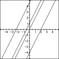
- Figure 1: Graphs of f(x) =y =2x+b for b=4.5; b=1; b=0 and b=-4.
Observe that as b changes the Y intercept of the lines also changes. This
makes sense, since for
x=0, f(0) = y =b, gives all the points of the form (0,b).
The next graph shows variations for m, for y = mx + 2:
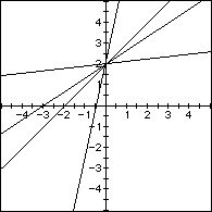
- Figure 2: Graphs of f(x) =y =2x+b for m=4.5; m=1; m=(2/3) and
m=(1/9).
Observe that for this set of graphs, the Y intercept is the same, at y=2;
values of m that are close to 0, make the line to tend to be horizontal.
values that are positive and big, will make the graph to tend to be a vertical
line, without being one, of course! As a general characteristic we can say
that these functions are always increasing. For negative values of m we
obtain a similar behavior, but now the functions will be decreasing; small
values of m will produce a kind of vertical line; values of m closer to
0 will produce a kind of horizontal line:
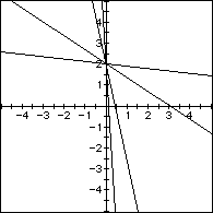
- Figure 3: Graphs of f(x) =y =2x+b for m=-4.5; m=-15; m=-(2/3)
and m=-(1/9).
A special case is obtained when m =0; in that case we obtain a horizontal
line. This background will be enough to understand the material that is
going to be presented in the next sections.
Addition of Two Linear Functions
Let f(x) = ax + k and g(x) = cx + d two linear functions defined on the
Real numbers.
The first operation that we can consider is the sum of two linear functions,
i. e. we want to consider the function h(x) = (f+g)(x), which is defined
as
h(x) = (f+g)(x) = f(x) +g(x).
Analytically, for our two functions we get h(x) = (a+c)x + (k+d). This
expression is of the form h(x) = mx +b, where the slope, m, is given by
(a+c) and the Y intercept, b, is given by (k+d). Observe that h(x) is a
horizontal line when a = -c; h(x) has a positive slope whenever a > -c
and h(x) has a positive Y intercept whenever k>-d. Some cases are illustrated
in Figure 4, Figure 5, and Figure 6.
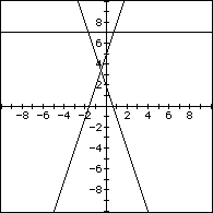
- Figure 4: Here f(x) = -3x + 2; g(x) = 3x + 5, h(x) = 7.
Here f(x) = -3x + 2; g(x) = 3x + 5 and h(x) = 7. Observe critical points
such as the ordered pair (-2,0) that belongs to g(x). For the same value
of x, f(x) is 7. Observe also that the functions intersect at -(1/2), and
then, as f(-1/2) =g(-1/2) = 7/2, h(x) = 2(7/2) =7. The next case also illustrates
the graphical meaning of the sum of two linear functions; in this example
f(x) =5 and g(x) = 2, and we are adding pointwise at x =-3:
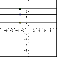
- Figure 5: Adding two functions term by term, for x = -3.
In the next example we have a line of positive slope, and positive Y intercept
that was obtained from the sum of two linear functions (an easier example
would correspond to adding a constant). The functions are f(x) =-3x +2;
g(x) = 4x +1. So h(x) = x + 3. The Figure 6 shows a pointwise sum at x =-1:
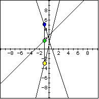
- Figure 6: are f(x) =-3x +2; g(x) = 4x +1. So h(x) = x + 3.
Product of Two Linear Functions
The next operation that can be considered is the product of two linear functions,
i.e. h(x) = (fg)(x), which is defined to be:
h(x) = (fg)(x) = f(x)g(x).
Analytically, for our special case, we obtain:

This expression always represents a parabola, except when ac is zero; in
such case we got an expression of the form h(x) = mx+b, with m=ad+kc and
b =kc For getting ac=0, we need to have either a, c or both equal to 0.
When both are 0, we obtain a horizontal line. When only one is zero, we
obtain a new non-vertical non-horizontal line, that has been transformed
by dilatation. Figure 7 and Figure 8 show some examples of these special
cases.
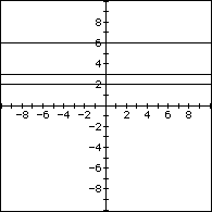
- Figure 7: f(x) =2; g(x) = 3; h(x) =6.
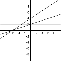
- Figure 8:

When we have ac different from 0, then we got a parabola. The parabola will
open upwards if ac is positive (so we need that both a and c have the same
sign); the parabola will open downwards if ac<0 (a and c has different
sign). Although our h(x) will be a parabola, h(x) will not represent all
the parabolas! Being the product of two linear functions, as it was said
before, the two linear functions will be zero for some value of x (at -k/a
and -d/c, for f and g respectively). That means that the product of the
two functions will vanish in at least one or in at most two values of x.
Then h(x) will represent all the parabolas such that the equation h(x) =0
has one or two solutions in the real numbers. This excludes the parabolas
that never intersect the X axis. This family of parabolas also happens to
have the property of intersecting the two original lines at least once p;exactly
at the X interceptsp; and at most twice; click here if you want
to see the case for which the lines intersect only once the resulting parabola,
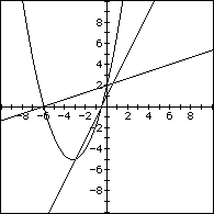
i.e. when they are tangent. Figure 9 and Figure 10 show some particular
cases illustrating what has been said.
- Figure 9:
 .
.
- Figure 10:

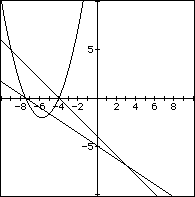
Observe that, for Figure 10 ac = 2/3 is positive, so the parabola opens
upwards; Observe also that having kd positive the parabola should have a
positive Y intercept. Observe also that the X intercepts of the line are
the X intercepts for the parabola. It is possible also observe that the
parabola is positive for the values of x in which f(x) and g(x) are both
positive (x>1) or negative (x<-6) and that the parabola is negative
when f and g have opposite signs (-6<x<1).
This reasoning may be helpful to construct a resulting parabola using only
the information given in a Cartesian plane. Consider for example the following
situation:
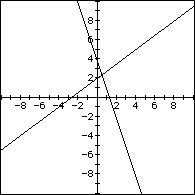
- Figure 11: Produce the parabola for the two given lines.
Suppose that we are given these graphs. What would be the resulting product?
We want to solve this question without using any symbolic reasoning. We
would like to use only the information on the Cartesian graph. First of
all we can highlight key points such as the X intercepts of the lines; lets
call these points A (the negative root), B (the positive root. Observe that
from A to B the lines are positive, then their product will be positive.
For other values, the functions will have opposite signs; so for other values
of x the parabola will be negative. We can sketch some possible parabolas:
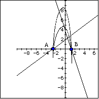
- Figure 12: Possible paths for the resulting parabola.
These two sketches are consistent with what was said about the sign of the
slopes. Since the slopes of the line have opposite signs, their product
will be negative, and the parabola will open downwards. Now will our parabola
be flat, and short? or thin and tall? We have a check point, for example
the Y intercept, C, of the parabola. Since both line intercepts are positive
and bigger than 1, it is clear that C has to be bigger than both intercepts
of the lines; this means that for this case C is bigger than 3; and being
the intercept of the second line near to 2, C will be close to 6. Another
check point is that the maximum of the parabola will be attained at the
midpoint between A and B; let's call it D. Since this point is less than
0, this means that h(D) is going to be bigger than our estimated C, although
it wont be too high. Figure 13 shows what would be an approximation for
the graph of the resulting h(x):
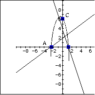
- Figure 13: Some key points.
How would we proceed to find the real h(x)? We would use the graphs for
estimating two points for each line and then use those points for defining
the equations of the lines. Once we got the equations, we will be able to
produce the parabola. For our case the resulting parabola is given below:
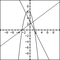
- Figure 14: The real parabola.
The functions were  .
.
Another particular case is obtained when f(x) = g(x). In this case we obtain
a parabola that has only one intercept in X:
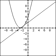
- Figure 15: Particular cases: f(x) = g(x).
Observe that in this particular case, we always obtain parabolas that opens
upwards, since we are squaring a expression, and a squared expression can
only be positive or zero.
What happens if the lines have different slope but the same intersection
point at the X axis? First of all our resulting parabola will have only
one root. It will open downwards if the slopes of our lines have opposite
signs, and upwards if they have the same sign:
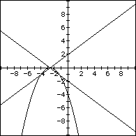
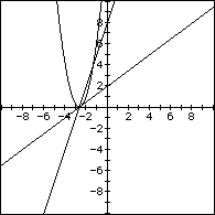
- Figure 16: Particular cases: Same intersection point.
Division of Two Linear Functions
Now we turn to consider  , which is defined as
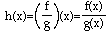 , for all x, such that g(x) be different from 0.
In our case,  . Let's consider some special cases. If a = c and k
= d, or more general if (ax+k) = M(cx+d), for some M a real number. then
h(x) = 1/M and corresponds to a horizontal line, that has a hole in the
value of x at which g(x) vanishes, i. e. The function is not defined when
x = -(d/c) (provided that c be different from0 also).
. Let's consider some special cases. If a = c and k
= d, or more general if (ax+k) = M(cx+d), for some M a real number. then
h(x) = 1/M and corresponds to a horizontal line, that has a hole in the
value of x at which g(x) vanishes, i. e. The function is not defined when
x = -(d/c) (provided that c be different from0 also).
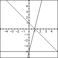
- Figure 17: f(x) =4x-4; g(x) = -x+1; h(x) = -4.
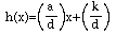
When c = 0, but d0, we got:
 ,
,
which is an equation of the form y = mx + b, so its analysis reduces
to the analysis of a linear function. Observe that in this case the domain
of the function is the Real numbers.
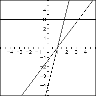
- Figure 18:
 .
.
In all other cases, we obtain that h(x) is a transformation of the function
j(x) = 1/x:
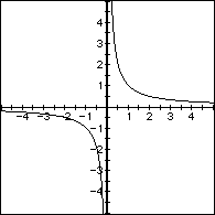
- Figure 19:

This is true, because we can write
 ,
,
and after some algebraic manipulations we got:

 ,
,
where 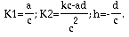
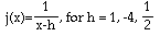
So, h represents a horizontal translation of  ; a translation to the
right when h>0, and a translation to the left, when h<0; Figure 20
represents some graphs of
; a translation to the
right when h>0, and a translation to the left, when h<0; Figure 20
represents some graphs of  for different values of h:
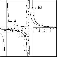
- Figure 20: Transformations of
 .
.
K1 represents a vertical translation of the graph; if K1 is positive, it
will be a translation upwards; for K1 negative will be a translation downwards.
Figure 21 represents some graphs for different values of K1:
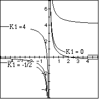
- Figure 21: Transformations of
 .
.
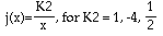
K2 is a dilation factor; Figure 22 represents the graph for several values
of K2.
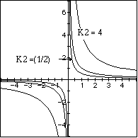
- Figure 22: Transformations of
 .
.
Composition of Two Linear Functions
Our last operation to consider is composition, h(x) = (fog)(x), which is
defined as
- h(x) = (fog)(x)=f(g(x))= a(g(x)) + k
- = a(cx+d) + k =
- = (ac)x + (ad+k)
which is, again, an expression of the form y = mx + b. So the composition
of two linear functions will be a function always.
The composition of two functions has an interesting graphical interpretation.
Let's consider first the case in which f(x) is of the form x+k, for k a
real number. Then h(x) = (cx+d) + k will be a vertical translation of k
units of the graph of g(x); upwards if k>0; downwards otherwise:
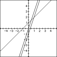
- Figure 23: f(x) = x + 1; g(x) = 3x -1; h(x) = 3x.
What is the expected outcome if instead of doing f(g(x)), we do g(f(x))
for this particular case? Analytically, we got g(x+1) = 3(x+1) -1. So graphically,
it would correspond to a movement of the graph of g(x) 1 unit to the left:
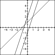
- Figure 24: g(x+1) = 3(x+1) -1
Let's consider what happens if f(x) =3x; then f(g(x)) = 3(g(x)), so, no
matter what function g(x) is, f(g(x)) will multiply it by 3. These three
last examples show how is it possible to model the translations of graphs
using linear functions; <click here if you want to see some transformations
of this kind when g(x) = sin(x)>.
The following sequence of functions will help to visualize why is this happening.
The graph on the left shows f(x); the one to the right shows g(x) and the
next one presents some points derived from making the composition between
the two functions.
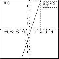
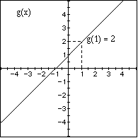
- Figure 25: Graphical production of f(g(1)).
g(1) =2; f(2) = 5; so f(g(1)) = 5, so the point (1,5) will belong to the
graph of f(g(x)); similarly, g(0) = -1; but f(-1) = 0. Then f(g(0)) = 0:
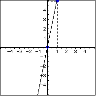
- Figure 26: Particular cases of f(f(x)), obtained graphically.
Concluding remarks
The study of linear functions from a graphical perspective can give us a
better understanding of their nature; exploring the possible operations
between two linear functions can help us to consolidate the concept of linear
function as objects which have certain properties and which can be manipulated;
I hope that this paper can present another view to the teaching of algebra
de functions, from a richer perspective; and that at least it help to see
possible strategies to analyze a similar situations with functions different
from the linear, or the nicely behaved polynomial functions.
Back to My Home Page
Return to EMT
668 Home Page