Department of Mathematics Education
EMT 669

Maria Gaetana Agnesi (1719-1799) of Milan was a gifted scholar and linguist who was first published at the age of nine with a Latin essay defending higher education for women. She was a well-published scientist by the age of 20 and was made an honorary member of the faculty at the University of Bologna with the consent of the pope at the age of thirty. She later retired to devote herself to her religious work. Her two volume textbook was the first comprehensive textbook on the calculus after L'Hopital's earlier book. She is most famous for her curve Agnesi called versiera, or turning curve. We know this curve by the name the "witch of Agnesi" because a British mathematician, John Colson, translated the word versiera incorrectly.
Investigations of the Witch Curve
The algebraic equation that generates this curve is
By substituting the values 1,2, and 3 in for a, we get the following graphs using Algebra Xpresser.
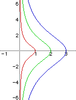
In order to "turn" the curve onto the x-axis, we take the inverse of the equation
and obtain the equation
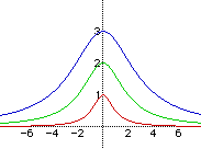
By substituting the same values for a and again using Algebra Xpresser, we can obtain the following graph.
We can also generate this curve using GSP. For the simplest example, we begin with a circle of radius 1 centered at (0,1) which gives us the curve represented algebraically above by a=2. To construct this curve, we first construct the aforementioned circle. The line y = 2, which is tangent to the circle at the point Q: (0,2), is constructed and a point anywhere on that line is chosen, call it point A. A segment is drawn from point A to the bottom point, O, of the circle (0,0). Where this segment OA intersects the circle we construct the point B. Then a line, l, parallel to y = 2 and through B is drawn and a line, m, perpendicular to l is constructed through point A. The intersection of l and m is point P. This is the point whose locus is traced, as A moves along
creating the witch curve.
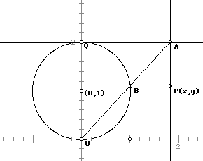
From this construction we can generate the parametric equations for the witch. We do this by expressing the coordinates of P in terms of t, the radian measure of the angle that segment OA makes with the positive x-axis. The following equalities, which we assume, and the figure below, aid us in this generation of parametric equations:
Equation i) is clear. AQ is the distance of point A from the y axis. Equation ii) follows from the definition of the sine function and triangle APB. The angle ABP has the same radian measure t as the line AO makes with the x-axis. Since A is on the line y = 2, the y-coordinate of P is give by 2-ABsin(t). Equation iii) follows from considering similar right triangles ABQ and AQO. Angle ABQ is a right angle because triangle OBQ is inscribed in a semicircle and angle ABQ is supplementary to angle OBQ. The acute angle at A is common to both triangles. Therefore they are similare and equation iii) follows.
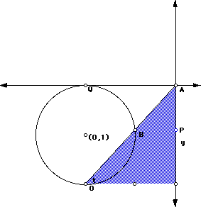
The construction highlights the triangle and the angle we are discussing throughout the proof.
The construction leads us to the equation tan(t) = y/x which in turn leads us to the fact cot(t) = x/y. Solving for x obtains the equation x = y cot(t) and as
we have the final parametric equation for x,
Now we wish to find the y equation. From (iii) we can see that
From the construction we know that OA is the hypotenuse of our proof triangle, so
By substitution,
which can we expanded to
which becomes
When this is then put into
we have
and this reduces to
From the trigonometric identity,
this equation becomes
Finally this reduces to the parametric equation
So, in conclusion, the general parametric equations for the witch are:
We can use these parametric equations in Theorist 2.0 to generate the witch curve as well.
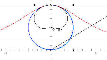
EXPLORING WITH GSP
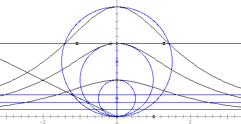
Returning to GSP, we can look at the expansion and contraction
of the radius of the original circle while keeping the line through
the point (0,2). This results in changes of the curve. When the
radius is expanded, the curve becomes steeper and when the radius
is contracted, the curve flattens out. Examples of this can be
seen below.
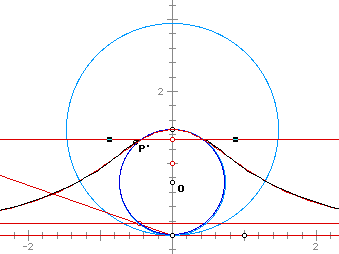
Another interesting investigation of the witch is the inversion of the curve. Looking at the original construction, we first chose the unit circle with center at (0,1) to be our point of inversion. We see as the witch curve expands towards infinity, the inversion tends towards the center point O.

If the unit circle with center at (0,0) is chose as the circle of inversion, and the circle for the Witch curve has radius 2, then the black curve below is the inversion of the red Witch curve.
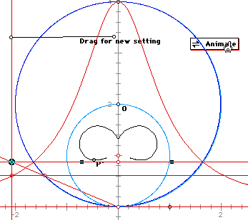
When the two circles are the same - -
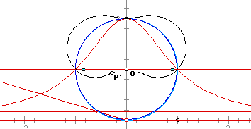
When the circle of inversion has as its radius the diameter of the circle for the Witch curve then the inversion corresponds to the the shape of the Witch curve. The example below has the generating horizontal line of the Witch curve in a strategic spot just under the end of the diameter. The result is a virtual overlap of the Witch curve and its inversion.
